Best available practice in life cycle assessment of climate change, stratospheric ozone depletion, photo-oxidant formation, acidification, and eutrophication-Backgrounds on specific impact categories | RIVM

(1)

RIVM report 550015003/2001

Best available practice in life cycle assessment of climate change, stratospheric ozone depletion, photo-oxidant formation, acidification, and eutrophication

Backgrounds on specific impact categories

W. Klöpffer, J. Potting (eds.), J. Seppälä, J. Risbey, S. Meilinger, G. Norris, L.G. Lindfors, and M. Goedkoop

This report is prepared by the SETAC Europe Scientific Task Group on Global And RegionaL Impact Categories (SETAC-Europe/STG-GARLIC) that is installed by the 2nd SETAC Europe working group on life cycle impact assessment. The report is published for the account of the Directiorate-General of the National Institute of Public Health and the Environment (RIVM), within the framework of project 550015.

(2)

Corresponding address:

Center for Energy and Environmental Studies IVEM University of Groningen Nijenborgh 4 9747 AG Groningen The Netherlands Telephone: 00 31 50 363 46 05 Fax: 00 31 50 363 71 68 Email: J.Potting@fwn.rug.nl

(3)

Abstract

This report has been prepared by the SETAC Europe Scientific Task Group on Global And RegionaL Impact Categories (SETAC-Europe/STG-GARLIC) that is installed by the 2nd SETAC Europe working group on life cycle impact assessment (WIA-2). This document is background to a chapter written by the same authors under the title “Climate change, stratospheric ozone depletion, photo-oxidant formation, acidification and eutrophication” in Udo de Haes et al. (2002)1_{. The chapter summarises the work of the STG-GARLIC and aims} to give a state-of-the-art review of the best available practice(s) regarding category indicators and lists of concomitant characterisation factors for climate change, stratospheric ozone depletion, photo-oxidant formation, acidification, and aquatic and terrestrial eutrophication. Backgrounds on a selection of general issues relevant in relation to LCA and characterisation of impact in LCA are given in another background reportfrom Potting and Klöpffer (2001)2.

1_{Udo de Haes, H.A., G. Finnveden, M. Goedkoop, M. Hauschild, E.G. Hertwich, P. Hofstetter, O. Jolliet, W.}

Klöpffer, W. Krewitt, E. Lindeijer, R. Müller-Wenk, S.I. Olsen, D.W. Pennington, J. Potting and B. Steen. Life-cycle impact assessment: Striving towards best practice. ISBN 1-880611-54-6. Pensacola (Florida, United States of America), SETAC-Press, 2002.

2_{Potting, J., W. Klöpffer (eds.), J. Seppälä, J. Risbey, G. Norris, L.G. Lindfors, and M. Goedkoop. Best}

available practice in life cycle assessment of climate change, stratospheric ozone depletion, photo-oxidant formation, acidification and eutrophication. Backgrounds on general issues. Report by SETAC Europe Scientific Task Group on Global And Regional Impact Categories (SETAC-Europe/STG-GARLIC). RIVM-report 550015002. Bilthoven (RIVM), National Institute of Public Health and the Environment (RIVM), 2001.

(4)

(5)

Preface

Methods like integrated modelling of the chain from cause to environmental effect are of growing importance for the support of European Environmental policy. RIVM explores the potential of broadening the basis of such integrated environmental assessment methods with knowledge and conventions applied in Life Cycle Assessment and Substance Flow Analysis in close collaboration with the Center for Environmental Science of the University of Leiden, and the dept. of Science, Technology and Society of Utrecht University, and SETAC3. We are therefore happy to publish this document as a RIVM report.

This document is prepared by SETAC’s Europe Scientific Task Group on Global And RegionaL Impact Categories (SETAC-Europe/STG-GARLIC) that is installed by the second SETAC Europe working group on life cycle impact assessment (WIA-2). This working group has adopted as a priority aim to establish best available practice(s) regarding impact

categories, category indicators, and equivalency factors to be used in impact in Life Cycle Assessment. Scientific Task Groups are formed around groups of impact categories to start this process. SETAC-Europe/STG-GARLIC deals with acidification, aquatic and terrestrial eutrophication, photo-oxidant formation, stratospheric ozone depletion and climate change. The ultimate aim is to develop general indicators that integrate environmental side-effects of economic activities, which can be used in decision-making by governments, companies and consumers.

Drs. Rob Maas

(Head of the Environmental Assessment Bureau of RIVM)

(6)

(7)

Samenvatting

Dit document geeft informatie over de karakterisatie van klimaatverandering, stratosferische ozonafbraak, formatie van foto-oxidanten, verzuring en aquatische en terrestrische

vermesting. Per milieu-effectcategorie wordt een overzicht gegeven van de stand van zaken met betrekking tot karakterisatie van deze categorie in LCA.

(10)

(11)

Summary

This document provides information about characterisation of climate change, stratospheric ozone depletion, acidification, troposheric photo-oxidant formation, and terrestrial and aquatic eutrophication. For each impact category, an overview of the state-of-the-art is given about characterisation of the given impact category in LCA.

(12)

(13)

1 Climate

change

(written by W. Klöpffer and S. Meilinger)

1.1 Background

The physical basis of this area of public environmental concern is the so-called greenhouse effect or, more specifically, the enhanced, anthropogenic greenhouse effect. The natural greenhouse effect, which has been known for more than hundred years, is mainly due to the gas carbon dioxide in its pre-industrial concentration and water vapour. The natural

greenhouse effect ensures higher life on earth, since without it the average temperature at the surface of the earth would be about -18oC, compared to the actual global average of +15oC. This actual average is due to the absorption infrared radiation sent back from the surface of the earth toward the space.

The additional or enhanced anthropogenic greenhouse effect, which in the last 100 years is considered by many scientists to have already caused an increase of the average surface temperature of about 0.5 to 1 oC [1], is due to the increase of the atmospheric concentrations of several trace gases, which are partly identical with the "natural" greenhouse gases:

• Carbon dioxide (CO2) • Methane (CH4) • Nitrous oxide (N2O)

• Synthetic, persistent, especially halogenated chemicals (e.g. tetrachloro- and tetrafluoromethane, sulfurhexafluoride).

The mechanism causing the warming effect is called “radiative forcing” and consists essentially in infrared absorption in the spectral region between 10 and 15 µm, the “spectral window” of the atmosphere. The enhanced radiative forcing and thereby enhanced global warming can be seen as the primary effect from the increase of greenhouse gases in the atmosphere.

Besides primarily emitted gases being greenhouse gases, greenhouse gases may also be produced as secondary products (e.g. ozone). Such secondary greenhouse gas formation can be due to natural as well as anthropogenic sources and contribute to the enhanced radiative forcing. In addition to gases, aerosol particles also have a radiative forcing effect which, depending on the particle properties, can have a positive or negative sign, leading to warming or cooling.

Several secondary and tertiary effects have been identified, which may follow the primary radiative forcing and warming, such as climatic instabilities (e.g. storms), increasing

(14)

sea-level, changing of oceanic streams etc. Therefore, the more general name “Climate change” replaced the formerly used “Greenhouse effect” as a description of the environmental theme and the impact category.

1.2 Climate change as an impact category

As an impact category, climate change was introduced into LCIA in the early 90’s [2,3]. The quantification proposed for this category is based on IPCC’s Global Warming Potentials (GWP) [1,3]. It became the model for quantifying or characterising most of the other impact categories. In the fundamental paper of WIA-2 [4], Climate change has been described as follows:

This category is generally known under the heading “global warming”; it can better be called “Climate change” because also storms or regional cooling can be part of the impacts. The modelling at the level of radiative forcing is rather well underpinned, less so impacts further along the impact network (displacement of Gulf Stream; release of methane from tundra’s?). Therefore there is as yet no basis for choosing the category indicator further along the impact network. It should be mentioned however, that in the ExternE programme modelling at the level of endpoints is taken (Eyre et al., 1997 [5]). The choice of the most appropriate time period has to be considered; depending on the choice to be made regarding the temporal aspects (see question in section 3.3).

Proposal:

a) Areas of protection: human health, natural environment, man-made environment b) Content of impact category: all impacts related to climate change caused by changes in

radiative forcing

c) Category indicator: radiative forcing

Climate change is an output-related impact category, describing global impacts [6] and many identified “endpoints”, some of them likely, others still speculative. The relevant gaseous emissions, quantified as mass per functional unit in the inventory, originate from many human activities, e.g.:

• burning of fossil fuels (CO2) • calcination of minerals (CO2) • agriculture (CH4, N2O)

• losses during extraction and transport of fuels (CH4) • industrial processes (chlorinated solvents, CF4, SF6, N2O) • private use (freons, chlorinated solvents)

(15)

Not quantified in life cycle inventory are CO2-emissions from burning or aerobic metabolism of renewable raw materials and fuels that have been produced recently from atmospheric CO2 via assimilation.This is not true, however, for methane formed anaerobically from the same sources, e.g. in landfills. This is due to the much higher Global Warming Potential (GWP) of methane relative to carbon dioxide, the end product of atmospheric oxidation of methane.

1.3 Positioning of the indicator

The positioning of the indicator between the “elementary flows” quantified in the inventory and the "endpoints" or potential effects within an impact category is free according to ISO 14042 [7c]. Selecting an indicator near to the elementary flows has the following advantages: • The endpoints have not to be known in detail, i.e. the causal chains have not to be

established quantitatively

• The indicators can often be defined rigorously and derived from basic laws

• The precautionary principle is in general better taken into account, since (still) unknown secondary and tertiary effects are automatically included if they are related to the primary effect and this primary effect is used for the indicator model. Even if some secondary effects are definitely known and may be modelled with a reasonably accuracy, other effects not known today may surface in the future.

• The number of effective categories is not increased by the introduction of subcategories (inevitable if several endpoints are modelled as indicators)

The main advantage of selecting the indicator near to the endpoints is the completeness of the analysis (at the present state of knowledge), especially if no common primary effect can be identified. In this case, however, the question is allowed whether the impact category itself has been selected and defined properly.

In the case of “Climate change” it is consensus within the community of atmospheric scientists that the midpoint “enhanced radiative forcing” (i.e. the absorption of infrared radiation in the spectral “window” from about 10 to 15 µm) is the common and global primary effect which may cause several serious secondary and tertiary effects whose actual regional consequences may dramatically endanger the future existence of humankind. The enhanced radiative forcing is linked to the “global warming”, i.e. the increase of the average temperature near the surface of the earth. That is why this impact category has formerly been called “Global warming”. For this reason and the general arguments given above, it is

advisable to select enhanced radiative forcing as the midpoint to be modelled and

characterised as the indicator for the renamed impact category “Climate change”. The new name, which implies a broader definition, gives the option of defining new indicators closer to the endpoint in the future, if atmospheric sciences sufficiently progressed in order to present simple and yet accurate calculations for well defined secondary or tertiary effects.

(16)

1.4 Selection of the indicator model and of characterisation factors

1.4.1 The global warming effect

As proposed in section 1.3, radiative forcing by (anthropogenic) emissions is the most appropriate midpoint for the impact category “Climate change”. For modelling purposes, however, the closely related global warming effect is used as the indicator.

Substances which are able to contribute to radiative forcing have to be sufficiently stable (persistent) in the troposphere and to have absorption bands in the spectral region between about 10 and 15 µm. Since both the absorption cross section (absorption coefficient) and the lifetime or persistence contribute to the effect, there is no simple way to calculate the global warming caused by a specific compound. Due to the effect of the lifetime which differs from compound to compound, a time-dependency becomes evident which is more pronounced for substances with relatively short lifetimes (e.g. methane [8]).

To complicate things further, several indirect effects have been identified which presently cannot quantified with sufficient precision. To give an example, the chlorofluorocarbons (CFC) show a pronounced radiative forcing due to strong absorption in the spectral window and high persistence; the depletion of the stratospheric ozone layer caused by these

substances (see chapter 2), however, is believed to have an indirect cooling effect and thus counteracts the warming effect due to radiative forcing [10]. Since this cooling effect cannot be quantified, the Intergovernmental Panel on Climate change (IPCC) decided to exclude the freons from the list of global warming gases in the 1996 Report [1c].

Since furthermore the prediction of temperature increases depends on the further

development of the emissions - especially of CO2 - and thus also on the measures taken (or not taken) in order to reduce the emissions, scenarios for this development enter into the calculations of further temperature increases and the contribution of the individual “greenhouse”-gases. Due to the scenarios, the different lifetimes of the gases and other related effects, a time dependence of the contributions is introduced into the results of the calculations, known as the “time horizon” of the Global Warming Potentials (GWP) to be discussed below.

1.4.2 The IPCC model

According to ISO 14042 [7c], the indicator model chosen for an impact category should ideally be based on scientific evidence and be supported by an international organisation. In the case of the category Climate change, the second condition is fulfilled by IPCC, working under the auspices of UNEP and WMO. The reports published by IPCC [1] are

peer-reviewed by a panel consisting of several hundred leading experts world-wide. For this reason, it can be assumed that the models and the results obtained are based on the best scientific evidence available at present. However, a fully objective scientific theory cannot be

(17)

expected presently due to assumptions in the scenarios needed, as mentioned in section 1.4.1. The unprecedented effort made by the scientific community, which is focussed in IPCC, guaranties that the best scientific evidence presently available is used and that the scenarios are realistic to the extent possible.

The models used by IPCC serve different purposes. One purpose is the prediction of future and the explanation of past temperature increases due to the anthropogenic greenhouse effect. Actually, the known development since the beginning of the industrialisation is used for the calibration of the models and their predictive power. A second purpose, which is of

paramount importance for the environmental policy, aims at proposing reduction rates and political and technical measures for the most important greenhouse-gas-emissions. For this purpose, different scenarios are calculated, showing the temperature increase after a given time horizon. A third purpose, which is the most important for LCIA, is to calculate the relative contribution of the different gases at the basis of equal weight. The question to be answered here is: how much more (or less) contributes one mass unit of gas A relative to one mass unit gas B to the global warming at a given time horizon.

The form chosen by IPCC for quantifying these ratios is ideally suited for the characterisation of Climate change or - actually the other way round - since the form given by IPCC is so well suited for LCIA, this form has been adopted as the general model of the characterisation of basically all impact categories [3]. The ratios calculated for different time horizons are called Global Warming Potentials (GWP) and are normalised with regard one mass unit of carbon dioxide. A GWP of 100 says that 1 kg of the substance has the same global warming effect (at a given time horizon, e.g. 100 years) as 100 kg CO2. It is immediately clear that a list of GWPs including those greenhouse gases quantified in the inventory [7b], allows the

aggregation of the masses per functional unit into one figure, the GWP [kg CO2-equivalents] per functional unit (f.u.).

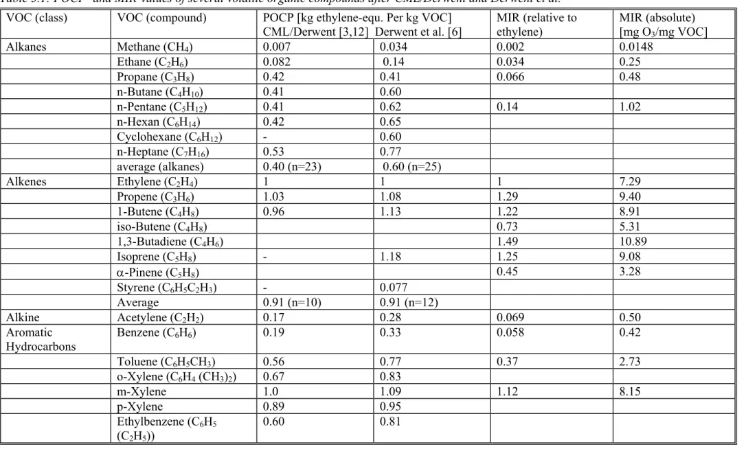
1.4.3 Numerical values of GWP for greenhouse gases

In Table 1.1, the GWPs of the most important greenhouse gases are presented for three time horizons. As can be seen from the data, the GWP of some compounds is several orders of magnitude higher compared to CO2 (GWP 103 to 104). The main overall contribution to global warming is nevertheless due to CO2 (61 % [1f]) due to its high anthropogenic emission (26000 Tg in 1990 [1f]). This is true in a global perspective; for certain product systems other greenhouse gases may be much more important.

(18)

Table 1.1: GWP and Lifetimes of Greenhouse Gases after IPCC and WMO [1c,10] in [kg CO2-equivalents/kg] and Lifetimes

Compound (i) Lifetime a

τi [years] Lifetime (OH) b τi [years] GWPi c Time Horizon 20 yr GWPic Time Horizon 100 yr GWPi c Time Horizon 500 yr Carbondioxide (CO2) determined acc. to

the Bern C-model

1 1 1

Methane (CH4) 8.9 ± 0.6 64 * 24 * 7.5 *

Dinitrogenoxide, nitrous oxide (N2O) 120 330 360 190 HCFC-22 (CHClF2) 11.8 12.3 5200 1900 590 HFC-23 (CHF3) 243 255 11700 14800 11900 HFC-32 (CH2F2) 5.6 2900 880 270 HFC-41 (CH3F) 3.7 460 140 43 HCF-125 (C2HF5) 32.6 6100 3800 1200 HFC-134 (C2H2F4) 10.6 3400 1200 370 HFC-134a (CH2FCF3) 13.6 14.1 4100 1600 500 HFC-152a (C2H4F2) 1.5 630 190 58 HCF-143 (C2H3F3) 3.8 1200 370 120 HCF-143a (CH3CF3) 48.3 6800 5400 2000 Sulphurhexafluoride (SF6) 3200 15100 22200 32400 CFC-11 (CCl3F) 45 > 6400 ** 6300 4600 1600 CFC-12 (CCl2F2) 100 > 6400 ** 10200 10600 5200 CFC-113 (C2Cl3F3) 85 6100 6000 2700 Dichloromethane (CH2Cl2) 0.4 to 0.5 35 10 3 Chloroform (CHCl3) ca. 0.5 55 16 5 Tetrachloromethane, Carbon tetrachloride (CCl4 ) 35 ≥ 130 ** 2100 1400 450 1,1,1-Trichloroethane, Methyl chloroform (CCl3CH3) 4.8 5.7 450 140 42 Tetrafluoromethane (CF4) 50000 3900 5700 8900 Hexafluoroethane (C2F6) 10000 7700 11400 17300 Perfluoropropane (C3F8) 2600 5900 8600 12400

(19)

Compound (i) Lifetime a τi [years] Lifetime (OH) b τi [years] GWPi c Time Horizon 20 yr GWPic Time Horizon 100 yr GWPi c Time Horizon 500 yr Perfluorobutane (C4F10) 2600 5900 8600 12400 Perfluoropentane (C5F12) 4100 6000 8900 13200 Perfluorohexane (C6F14) 3200 6100 9000 13200

a Tropospheric residence time after [10] or [1c]; in case of non-coincidence the more recent value is given [10]

b Tropospheric chemical lifetime calculated from the rate constant of reaction with OH-radicals and average OH-concentration in the troposphere; data after IPCC 1996 [1c] and WMO 1999 [10]. The tropospheric (OH) lifetime gives an upper limit for the tropospheric

residence time, since all degradation- and other (physical) removal processes shorten the average time spent by a molecule in the troposphere c Most recent data after WMO 1999 [10]; in this compilation of direct GWPs more data on CFCs, HFCs and other halogenated compounds are available. The data of CH4 and N2O are basically those of IPCC 1996 [1c], but re-scaled according to new scientific evidence. IPCC 1996 [1c]

does not include substances degrading the stratospheric ozone; they are included in IPCC 1990 [1a] and WMO 1999 [10]; the values given here [10] are typically 10 to 20% higher compared to [1a]

* Includes indirect effects as tropospheric ozone formation and stratospheric water formation

** Calculated according to experimental kOH-values [9] at 298 K; actual lifetimes are higher due to the lower average temperature of the

(20)

The time horizon chosen for the calculation influences the GWP values significantly only in the case of relatively short lifetimes (up to about 100 years). The typical uncertainty of the GWP of individual greenhouse gases is in general about ± 35 %. Since GWPs of individual gases are relative numbers, this uncertainty does not contain the absolute uncertainty of climate modelling of carbon dioxide; this, however, is no concern to LCIA since only relative values are necessary in the indicator model chosen.

In Table 1.1 some GWP-values of persistent chlorinated gases are included. As discussed in section 1.4.1, using these data may overestimate the GWP, since the compensating effect is not taken into account. Their use or not-use in a specific LCA has to be discussed in the goal and scope definition of that study. It may be argued that the precautionary principle is better fulfilled if the GWP of chlorofluorocarbons (CFC, freons) and chlorinated persistent solvents is taken into account, although the calculated total GWP may be too high.

1.4.4 Selection of the time horizon

For principal reasons, a large time horizon should be chosen in LCIA [4] in order to prevent a too restricted impact assessment, not taking into account possible negative effects for the coming generations. For this reason, the longest horizon used in the calculations (500 years) would be appropriate. However, scenarios defined today are very unlikely to hold true for the future and seem to be most accurate for the time being. It may therefore be a good

compromise to use GWP data calculated for a time horizon of 100 years, as has been done in most LCIAs in the past.

For special LCAs, dealing explicitly with products under the aspect of, e.g. reducing global warming, a more detailed handling of this question may be necessary. In these cases, the goal definition may include requirements for using several time horizons or, at least, to include the uncertainty introduced by using one fixed time horizon.

1.4.5 Calculation of the indicator result

The formula used for calculating the indicator result from the inventory data classified for the impact category “Climate change” is given in equation (1.1).

GWP = ∑i (mi x GWPi) (1.1)

GWP: Indicator result for the impact category Climate change [kg CO2-equivalents/functional unit]

mi: Mass of greenhouse gas i assigned to the impact category Climate change during “classification” [kg i /functional unit]

GWPi: Global warming potential of gas i [kg CO2 equivalents/kg i] for time horizon 100 years (if not otherwise requested)

In using (1.1) the most recent list of GWPi -values published by IPCC or WMO should be used. The data selection in Table 1 taken from WMO 1999 [10].

Due to the long lifetime of all greenhouse gases (the inter-hemispheric exchange time is in the order of one year), a good mixing in the troposphere can be expected. Therefore, as an

(21)

1.5 Further developments and recommendations

In the future, reliable calculations linking the emission of greenhouse gases with potential secondary effects of global warming may become possible (see [5,8]). Depending of the goal definition, such indicators nearer to endpoints affecting human life and ecosystems more directly than radiative forcing as such may be useful in LCA to facilitate weighting across impact categories. Radiative forcing itself is not well suited as an indicator for aggregating the climatic effects of emissions since the lifetime of the molecules does not enter into the

calculation [10]. The closely related global warming effect is therefore a much better indicator and should be retained in LCIA.

Considering the rules given by ISO 14042 [7c], indicators nearer to the endpoints may be used in special LCAs. For the time being, however, we propose to practitioners to use • The IPCC global warming model as the indicator model which is based on radiative

forcing

• A time horizon of 100 years, if not required otherwise in the goal definition of the LCA • The latest GWPi-list published by IPCC or WMO, and

• Equation (1.1) for calculating the indicator result

Atmospheric/environmental researchers and LCA-developers should • Provide GWPi-values for all chemicals persistent in the troposphere

• Investigate the indirect effects (including particles) and provide modified GWPi-values where necessary

• Investigate the effect of changing time horizons in real-life LCAs

• Consider requirements for the inventory (greenhouse gases not generally contained in present-day inventories, CH4 from anaerobic processes et cetera)

As in the case of the other impact categories, Climate change should be developed further and adjusted to the scientific progress that is fast in this area. Care should be taken, however, not to complicate more than necessary this category and the indicator recommended which for the reasons given is ideally suited for LCIA.

1.6 References

[1] IPCC: World Meteorological Organization (WMO)/United Nations Environment Programme (UNEP) - Intergovernmental Panel on Climate Change:

[1a] Climate Change 1994; Radiative Forcing of Climate Change and an Evaluation of the IPCC IS92 Emission Scenarios. Cambridge University press 1995

[1b] Climate Change 1995; The IPCC Synthesis. Cambridge University Press 1995 [1c] Houghton, J.T.; Meira Filho, L.G.; Callander, B.A.; Harris, N.; Kattenberg, A.;

Maskell, K. (Eds.): Climate Change 1995; The Science of Climate Change. Cambridge University Press 1996

(22)

[1d] Climate Change 1995; Scientific-Technical Analyses of Impacts, Adaptations, and Mitigation of Climate Change. Cambridge University Press 1995 (?)

[1e] Bruce, J.P.; Lee, H.; Haites, E.F. (Eds.): Climate Change 1995; The Economic and Social Dimension of Climate Change. Cambridge University Press 1996

[1f] Houghton, J.T.; Jenkins, G.J.; Ephraums, J.J. (Eds.): Climate Change. The IPCC Scientific Assessment. ISBN 0-521-40720-6 (paperback). Cambridge University Press, Cambridge 1990 (reprinted 1991 and 1993)

[1g] Intergovernmental Panel on Climate Change. IPCC Second Assessment Synthesis of Scientific-Technical Information Relevant to Interpreting Article 2 of the UN

Framework Convention on Climate Change 1995 (abridged version of the final draft Synthesis) ESPR - Environ. Sci & Pollut. Res. 3 (1996) 52-57

[1h] Houghton, J.T.; Callander, B.A.; Varney, S.K. (Eds.): Climate Change. 1992. The Supplementary Report to the IPCC Scientific Assessment. Cambridge University Press, Cambridge 1992 (reprinted 1992 and 1993).

[2] SETAC-Europe (ed.): Leyden Workshop Progresses LCA. LCA Newsletter 2 , No 1 (1992) 3-4.

[3] Heijungs, R.; Guinée, J.B.; Huppes, G.; Lamkreijer, R.M.; Udo de Haes, H.A.;

Wegener Sleeswijk, A.; Ansems, A.M.M.; Eggels, P.G.; van Duin, R.; de Goede, H.P.: Environmental Life Cycle Assessment of Products. Guide (Part 1) and Backgrounds (Part 2) October 1992, prepared by CML, TNO and B&G. Leiden 1992. English Version 1993.

[4a] Udo de Haes, H.A.; Jolliet, O.; Finnveden, G.; Hauschild, M.; Krewitt, W.; Müller-Wenk, R.: Best Available Practice Regarding Impact Categories and Category Indicators in Life Cycle Impact Assessment. Part 1. Int. J. LCA 4 (2) (1999) 66-74. [4b] Udo de Haes, H.A.; Jolliet, O.; Finnveden, G.; Hauschild, M.; Krewitt, W.;

Müller-Wenk, R.: Best Available Practice Regarding Impact Categories and Category

Indicators in Life Cycle Impact Assessment. Part 2. Int. J. LCA 4 (3) (1999) 167-174. [5] Eyre, N.; Downing, D.; Hoekstra, R.M.; Rennings, K.; Tol, R.: Global Warming

Damages. ExternE-Global Warming Sub-Task. Final Report to the European Commission, Contract JOS-CT95-0002 (1997).

[6] Udo de Haes, H.A. (ed.): Towards a Methodology for Life Cycle Impact Assessment. ISBN 90-5607-005-3. SETAC-Europe, Brussels, September 1996.

[7] ISO International Organization for Standardization, Environmental Management - Life Cyccle Assessment 14040ff.

[7a] International Organization for Standardization (ISO) Technical Committee TC 207/Subcommittee SC 5: Environmental management - Life cycle assessment - Principles and framework. International Standard ISO EN 14040, 1997.

(23)

[7b] International Organization for Standardization (ISO) Life cycle assessment - Goal and scope definition and inventory analysis. International Standard ISO EN 14041, 1998. [7c] International Organization for Standardization (ISO) Life cycle assessment - Life

cycle impact assessment. International Standard ISO EN 14042, 2000. [7d] International Organization for Standardization (ISO) Life cycle assessment -

Interpretation. International Standard ISO EN 14043, 2000.

[8] Graßl, H.: Global Climate Change. Bunsen-Magazin 1 (1999) 148-155.

[9] Atkinson, R.: Kinetics and Mechanisms of the Gas-Phase Reactions of the Hydroxyl Radical with Organic Compounds. J. Phys. Chem. Ref. Data Monograph 1, Am. Inst. Physics, New York 1989.

[10] WMO (1999) Scientific Assessment of Ozone Depletion: 1998. World Meteorologic Organization. Global Ozone Research and Monitoring Project - Report No. 44. Geneva 1999.

(24)

(25)

2 Stratospheric ozone depletion

(written by W. Klöpffer and S. Meilinger )

2.1 Introduction

The environmental concern about the impact category “Stratospheric ozone depletion” is based on the UV-absorption capacity of the ozone present in the stratosphere, which hinders radiation below 300 nm from reaching the troposphere and the surface of the earth. The ozone molecules are present in the stratosphere in very low concentration, but the layer thickness to be passed by the photons is very large (about 25 km), so that the absorption of short

wavelength radiation is complete despite the small concentration of O3. This absorption capacity, among other beneficial properties of the stratospheric ozone layer is at stake if ozone is depleted by anthropogenic emissions.

According to Chapman (1930), formation and decay of O3 in the stratosphere are in a dynamic equilibrium (2.1, 2.2): Formation of Ozone: O2 + hν ---> 2 O (λ = c/ν < 240 nm) (2.1a) O + O2 (+M) ---> O3 (+M) (2.1b) Destruction of Ozone: O + O3 ---> 2 O2 (2.2a) O3 + hν ---> O + O2 (λ = c/ν < 1140 nm) (2.2b) In addition to these reactions there are several additional formation- and degradation

processes going on, which are catalysed by trace constituents of the atmosphere (HOx, NOx). As early as 1970, the possible depletion of the ozone layer by supersonic jets emitting NOx during flights in the lower stratosphere have been discussed. An extension of this work to the ClOx cycle, which was new at that time, by Rowland and Molina was presented in two papers (1974, 1975 [1,2]) which had a high impact. In this work, a possible connection between the emission of freons or chlorofluorocarbons (CFC) and the postulated ozone depletion has been outlined and supported with reasonable data and assumptions.

Chlorine cycle of the catalytic ozone degradation [1], equation (2.3):

Cl + O3 ---> ClO + O2 (2.3a) O3 + O ---> 2 O2 (2.3b) ClO + O ---> Cl + O2 (2.3c) 2 O3 ---> 3 O2

The chlorine atom needed for initiating this cycle (2.1a) stems from the photolysis of

(26)

These compounds are able to penetrate the stratosphere, since reactions in the troposphere and washout processes (high Henry coefficient) are inefficient. Since the crossing of the

tropopause is a slow process (characteristic time about 10 years for substances emitted at the surface of the earth), there is a time lag between emission and effect.

In addition to this mechanism of homogeneous catalysis, which leads to a more or less equal and slow depletion of stratospheric ozone around the globe, the so called “ozone hole” was detected over Antarctica 1985 [4] and found to be due to heterogeneous catalysis [5-7]. It is important to know that this effect was not predicted by Roland and Molina`s theory, although the chemicals causing it are the same. This shows the importance of the precautionary

principle and our limited knowledge of complex reactions in the environment.

The heterogeneous reactions take place at acidic hydrate or ice particles and ternary solution droplets present in the lower stratosphere during the Antarctic winter and, to a lesser degree, also during the arctic winter. The effect is observed during Spring when the solar radiation liberates chlorine. Since the temperatures are lower in the Antarctic stratosphere, the effect is more pronounced there compared to the Arctic and thus has been detected earlier. According to a recent report by WMO [13] it was a series of exceptionally cold winters which increased the springtime ozone hole over the Arctic.

2.2 Stratospheric ozone depletion as an impact category

The impact category “Stratospheric ozone depletion” was introduced into LCIA together with the first list of categories and based on the “Ozone Depletion Potentials” (ODP) from the beginning [8]. In the basic paper of WIA-2, this category is described as follows:

Depletion of the stratospheric ozone layer leads to an increase of UV-B intensity at the surface of the earth, causing a number of radiation impacts: on algae and arctic flora, on crops, on wildlife and on humans. The first three are as yet rather uncertain; the latter can already be modelled with considerable certainty (cf. Müller-Wenk, 1997 [10]). As to the time period, a choice has to be made, depending on the choice to be made in section 3.3. In as far as relevant, possibly new modelling of background concentrations is necessary due to envisaged emission reduction.

Proposal:

a) Areas of protection: human health, natural environment, man-made environment, natural resources

b) Content of category: all impacts due to Stratospheric ozone depletion (including possible impacts on human health)

c) Category indicator: stratospheric ozone depleting potency of substances; in addition it will be analysed whether impacts on human health can be modelled in a comparable way to the human toxicity indicators.

Stratospheric ozone depletion is an output-related impact category, describing global and regional impacts due to the increased UV-radiation below about 300 nm. This radiation carries more energy per photon compared to the UV-radiation reaching the surface of the earth with an intact ozone layer. Therefore, many possible adverse effects can occur, leading to a multitude of potential endpoints from potential human toxicological effects to

(27)

The relevant gaseous emissions, quantified as mass per functional unit in the inventory, originate from many human activities, e.g.:

• aerosol sprays

• polymer foam production (e.g. polyurethanes)

• cooling agents for refrigerators and small air conditioners (cars) • cleaning agents (e.g. in the electronic industry)

• smaller applications in medicine (asthma sprays), analytical chemistry (extraction agents, solvents for IR-spectroscopy) et cetera

• fire extinguishing (Halons) • agriculture, pesticides (CH3Br)

Most of these uses have in the past been performed with CFCs and similar chlorinated

solvents. The majority of these chemicals are now forbidden in the industrialised countries as a consequence of the Protocol of Montreal (1987) and its subsequent adjustments and

amendments of London (1990), Copenhagen (1992), Vienna (1995) and again Montreal (1997) [13]. For some uses there are exceptions from the general ban; this together with the production going on in developing countries, some smuggling etc. causes still emissions of freons and similar ozone depleting substances. Some of the substitutes for CFCs might cause similar problems as well.

These facts have to be considered in the inventory component of LCA. The reference year of the data is especially important, since production and use of ozone depleting substances has changed dramatically in the last years.

2.3 Positioning of the indicator

The reasons for positioning the indicator near to “elementary flows” have been given in Section 1.3 for “Climate change”; they are equally valid for “Stratospheric ozone depletion”, since the secondary effects and possible endpoints are equally uncertain. This is especially true for damages of ecosystems and species exposed to solar radiation (air, surface waters, and oceans near to the surface, vegetation, surface of bare soils).

There is one effect that is reasonably well known in order to be considered as a separate endpoint: human skin cancer as a consequence of increased UV-B radiation. UV-B is the medical expression for this part of the solar radiation that is near to the natural edge at 290-300 nm. This part of the spectrum is the one that increases in intensity due to Stratospheric ozone depletion. Thus, in principal, a causal chain can be constructed which links the emission of ozone depleting substances with increased UV-B radiation and the likelihood of skin cancer incidents.

Two different situations have to be considered, however:

• the general increase of UV-B intensity due to photolyses of long-lived organic chlorinated compounds initiating the Rowland and Molina mechanism (homogenous catalysis)

• the temporary and regional increase of UV-B radiation during “ozone hole” events in the most southern and to a smaller degree also in the most northern regions of the globe during the southern or northern early springtime.

It should however be noted that the global effect of homogeneous ozone depletion is less severe with respect to increasing UV-B radiation than the regional ozone hole effect.

(28)

The common primary effect of Stratospheric ozone depletion is the increased ozone destruction in itself. Increased UV-B radiation at the surface of the earth is already a

secondary effect, and not the only one. Since absorption of solar radiation (not only UV) by stratospheric ozone contributes significantly to the warming of the stratosphere (the

tropopause being the thermocline between the stratosphere and the colder upper troposphere), ozone depletion may also cool the stratosphere and possibly change the stratification of the atmosphere. Possible tertiary effects from this are not calculable and belong into the realm of “Climate change”.

Due to the unforeseeable consequences of the primary ozone depletion (both

global/homogeneously catalysed and ozone-hole type/regional/heterogeneously catalysed) it is suggested to position the indicator near the elementary flows. As discussed for the closely related category "Climate change", the precautionary principle is best taken into account in that way.

2.4 Selection of the indicator model and of characterisation factors

2.4.1 The ozone depletion effect

As discussed in the proceeding sections, Stratospheric ozone depletion by halogen (chlorine- and bromine-) containing molecules occurs by two related but different mechanisms

• homogeneous catalysis (less important) • heterogeneous catalysis (more important)

where the first mechanism can occur globally in the whole stratosphere (although depending on the height and latitude) and the second one only temporarily during the Antarctic (and, to a minor degree, also arctic) spring. The common link between the mechanisms is the

intermediate ClO (and BrO), the main difference consists in the formation of this active species.

In order to be active as halogen (Cl,Br) carriers, organic substances have to be persistent (tropospheric lifetimes of several years) in order to reach the stratosphere before degradation occurs on the way up. This precondition is ideally fulfilled in perhalogenated compounds, e.g. CFC-11 (chlorotrifluoromethane) and CFC-12 (dichlorodifluoromethane) and to a minor degree also in partially halogenated compounds, as methylchloroform (1,1,1-trichloroethane) or methylbromide.

Fluor as substituent is not active per se, but increases the persistence by lowering the OH-reaction rate. Freon (CFC) substitutes have therefore be chosen among the fluorocompounds with residual H-atoms in order to enable the reaction with OH-radicals (HFC). As shown in chapter 1, however, the residual persistence in connection with IR-absorption is sufficient for the global warming effect.

2.4.2 The WMO-model

According to ISO 14042 [11], the indicator model chosen for an impact category should ideally be based on scientific evidence and be supported by an international organization of high reputation. In the case of the category “Stratospheric ozone depletion”, the second condition is fulfilled by the Global Ozone Research and Monitoring Project of the World Meteorological Organization (WMO), the United Nations Environment Program (UNEP) and other national and international bodies, [12,13]. The scientific evidence accumulated within

(29)

this program endorses the causal relationships outlined in the proceeding chapters, i.e. the halogen input by man-made persistent Cl- and Br- containing chemicals and the catalytic destruction of the stratospheric ozone.

As in the case of “Climate change”, modelling plays a major role in predicting the further development of the ozone layer as a function of the further development of the critical emissions and for identifying and quantifying the contributions of the individual substances which cause the adverse effects. It is this latter point which makes the models applicable to LCIA. Two basic models were developed in order to quantify the ozone depletion capacity of chemicals [12]:

• Chlorine Loading Potential (CLP) [14] • Ozone Depletion Potential (ODP) [15]

The CLP is the simplest model and considers only tropospheric lifetimes of the compound (relative to CFC-11), the molar mass and the number of Cl-atoms in the molecule considered. Since bromine is also - and even more - effective in degrading ozone, a Bromine Loading Potential (BLP) was defined in an analogous manner. The ozone depletion efficiency in the stratosphere, however, does not only depend on the factors included in the calculation of CLP and BLP, but also on the stratospheric lifetime which is controlled mainly by photolysis, not by the OH-reaction which dominates the tropospheric degradation of organic chemicals. Hence, the Ozone Depletion Potential (ODP) has been defined as a relative measure of the ozone depletion capacity [15] which avoids the deficiencies of CLP and BLP and allows the description of chlorine- and bromine-containing molecules in one parameter. The ODP is - in analogy to the older parameters - a relative number and uses the ozone depletion capacity of CFC-11 (trichlorofluoromethane) as a reference.

The ODP is defined by equation (2.4) [12]:

ODPi = (Global ∆ O3 due to i) / (Global ∆ O3 due to CFC-11) (2.4) ODPi: Ozone Depletion Potential of compound i

The verbal definition reads [13]:

The ODP represents the amount of ozone destroyed by emission of a gas over the entire atmospheric lifetime (i.e. at steady state) relative to that due to emission of the same mass of CFC-11, and is defined in modelling calculations as [see equation (2.4)].

It is clear from the discussion above that the ODP is superior to the chlorine and bromine loading potentials, since it allows to characterise both chlorine- and bromine- containing molecules in one parameter and includes differences in stratospheric as well as tropospheric lifetimes. Its determination requires models, however, whereas the loading potentials can be calculated from basic chemical knowledge and the OH-reaction rate constant. Several

atmospheric models were used for the calculation of ODP-values [13] resulting in similar, but not identical ODPs. The uncertainty is in the range of 20 to 50 %.

(30)

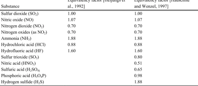
Table 2.1: ODPi of some ozone depleting gases after World Meteorological Organization [13]

Compound (i) Lifetime a

τi [years] Lifetime (OH) b

τi [years] ODPi (kg CFC-11 Equivalents per kg i) CFC-11, Trichlorofluoromethane (CCl3F). Reference substance 45 < 6400 1.0 CFC-12, Dichlorodifluoromethane (CCl2F2) 100 < 6400 0.82 CFC-113, Trichlorotrifluoroethane, (CCl2FCClF2) 90 0.90 CFC-114 1,2-Dichloro-1,1,2,2-terafluoroethane (CF2Cl CF2Cl) 0.85 CFC-115 1-Chloro-1,1,2,2,2-pentafluoroethane (CF2ClCF3) 0.40 Tetrachloromethane (CCl4) 35 > 130 1.20 Methylchloride (CH3Cl) ca. 1.3 1.3 0.02 HCFC-22, Chlorodifluoromethan (CHClF2) 11.8 12.3 0.034 HCFC-123, 2,2-Dichloro-1,1,1-trifluoroethane (CF3CHCl2) 0.012 HCFC-124, 2-Chloro-1,1,1,2-tetrafluoroethane (CF3CHClF) 0.026 HCFC-141b, 1,1,-Dichloro-1-fluoroethane (CFCl2 CH3) 9.2 10.4 0.086 HCFC-142b, 1-Chloro-1,1-difluoroethane (CF2Cl CH3) 18.5 19.5 0.043 1,1,1-Trichloroethane, (CH3CCl3) 4.8 5.7 0.11 Halon 1301, Bromotrifluoromethane (CBrF3) 65 12 Halon 1211, Bromochlorodifluoromethane (CBrClF2) 11 5.1 Halon 2402, 1,2-Dibromo-1,1,2,2-tetrafluoroethane (CBrF2CBrF2) 6.0 Methylbromide (CH3Br) 0.7 1.8 0.37 (0.2-0.5)

a Tropospheric residence time after [13]

b Tropospheric chemical lifetime calculated from the rate constant of reaction with OH-radicals and average OH-concentration in the troposphere; data after WMO 1999 [13]. In Table 2.1 a selection of numerical ODP values are given from recent sources. Due to the refereeing process of the WMO/UNEP-reports they may be considered as the best available figures at present. Future improvements and adjustments are likely and should be taken into account in actual LCIAs.

(31)

2.4.3 Numerical values of ODP for ozone depleting gases

As can be seen from the data, the highest values are those of the halons due to the about tenfold catalytic activity of bromine, compared to chlorine. The other perhalogenated compounds (Cl,F) are in the range of ODP 0.5 to 1.1. Compounds containing H-atoms that can react with OH in the troposphere and are therefore less persistent show much smaller ODP-values. The ODP-values of compounds containing only F as halogen are zero by definition, since F does not catalyse the ozone destruction. Iodine acts as catalyst, but I-containing compounds have a very short tropospheric lifetime due to photolysis (hours to a few days [13]) and therefore only a very small fraction enters the stratosphere.

2.4.4 Selection of the time horizon

The ODP-values given in Table 2.1 are calculated for the steady-state over a time horizon that is theoretically infinite. Since, however, the input into the environment of many compounds is not constant but changes rapidly due to the enactment of the protocol of Montreal and its amendments, this time horizon does not reflect a good representation of the “real” value. The question of time-dependency is discussed in [22]. According to this discussion, ODP (stationary) values of relatively short-lived compounds (e.g. HCFCs) are small, since they are derived with regard to CFC-11 whose steady-state - assuming constant emissions - will be reached in centuries. The short-term impact of not highly persistent ozone depleting

substances is therefore underestimated. If ODP is calculated for a short time-horizon of a few years, the ODP of relatively short lived compounds may be higher by an order of magnitude (but still smaller than that of CFC-11 due to the shorter tropospheric lifetimes).

In LCAs in which the goal definition specifically involves the comparison of different agents including freons and their substitutes, the time dependency should be taken into account. Time-dependent ODPs have been calculated for the most important compounds and a formula for the calculation is given [22]. For LCAs not dealing specifically with such problems, stationary ODP-values should be used. The data given in Table 2.1 is only an extract of ODPs available.

2.4.5 Calculation of the indicator result

The formula used for calculating the indicator result from the inventory data classified for the impact category “Stratospheric ozone depletion” is given in equation (2.5).

ODP = ∑i (mi x ODPi) (2.5)

ODP: Indicator result for the impact category Stratospheric ozone depletion [kg CFC-11 equivalents/functional unit]

mi: mass of ozone depleting gas i assigned to the impact category Stratospheric ozone depletion during “classification” [kg i /functional unit]

ODPi: ozone depletion potential of gas i [kg CFC-11 equivalents/kg i] for steady state (if not requested otherwise)

The ODPi-values should be taken from the most recent WMO/UNEP report. If time-dependent data are used, the model used for the calculation should be given.

(32)

Due to the long lifetime of most ozone depleting gases, a good mixing in the troposphere can be expected. Therefore, as an approximation for LCIA, no regional dependence of emissions has to be taken into account. This is also true if secondary effects (e.g. UV-B exposure of humans) should be considered. Whereas the effects show spatially differentiation (“ozone hole”), the responsible agents still distribute globally after emission and the spatial

differentiated effects can thus not be traced back to a specific region of emission. In case of quantifying secondary effects, other indicators have to be defined, which are not considered in this chapter.

2.5 Ozone depletion not related to Halogens

As mentioned in section 2.1, environmental concerns about ozone depletion by NOx preceeded the now accepted mechanism of halogen-induced stratospheric ozone depletion. The entrance path considered in the early 70’s was air traffic by supersonic aircraft [23]. This is still or again a matter of concern, since plans exist for a new generation of supersonic passenger aircraft.

The main source of nitrogen oxides in the stratosphere is N2O that has natural as well as anthropogenic sources [13,22,17]. N2O is highly persistent in the troposphere, (non polar molecule, no chemical sink) and thus reaches the stratosphere. The total column mixing ratio increased from 299 ppbv in 1976 to 310 ppbv in 1993, the growth rate is 0.2 to 0.3 % per year (3.1-4.7 Tg N/yr) [22]. The anthropogenic sources are not yet well understood, but nitrogen fertilising seems to play a major role [17]. In addition, some industrial processes (polyamide 66 and nitric acid production) contribute to the N2O emissions.

In the stratosphere N2O forms NO and secondary reactive NO-species which can degrade ozone by a well known catalytic mechanisms [24]. This mechanism is shown in equation (2.6): NO + O3 ---> NO2 + O2 (2.6a) O3 + hν ---> O + O2 (2.6b) NO2 + O ---> NO + O2 (2.6c) --- 2 O3 + hν ---> 3 O2

This mechanism of ozone depletion prevails in the middle stratosphere (25-35 km).

At lower altitudes, however, where the concentration of free oxygen atoms is lower, photo dissociation of NO2 (NO2→NO + O for λ=c/ν<405 nm) exceeds reaction (2.6c) and a photochemical equilibrium between O3, NO and NO2 establishes.

At even lower altitude, in the region of the tropopause (in the upper troposphere and the lowest part of the stratosphere), photosmog chemistry (see Chapter 3) might give rise to ozone production and to the oxidation of CO, CH4 and other hydrocarbons. Detailed studies by Ehhalt and Rohrer (1995) [18], Brasseur et al. (1996) [19] and Grooß et al. (1998) [20] show that the formation and decay of ozone in this region depends in a non-linear way on the availability of NOx. Further influencing factors are ozone, water, CO, hydrocarbons and solar radiation, all of which have strong gradients at the tropopause. An additional complication is given by heterogeneous chemistry on cirrus cloud particles. Depending on the local and temporal conditions, ozone depletion as well as ozone formation may prevail.

(33)

A further influence of NOx on the ozone dynamics in the lower stratosphere consists in the formation of reservoir species (e.g. HNO3 from NO2 and OH). These reservoir species slowly regenerate NOx by photolysis and OH. Active halogen species may also be stored as relatively inactive species, which can, however, be activated by heterogeneous catalysis and contribute to ozone degradation in the ozone-hole formation. Thus, the increase of nitrogen compounds may decrease the global ozone destruction, however, it’s removal in the polar regions (e.g. via washout into the troposphere) might increase ozone destruction by the heterogeneous

mechanism.

The effect of NOx by aircraft depends on the altitude. Subsonic aircraft fly at altitudes of 9-13 km and thus partly in upper troposphere (circa 60 %) and partly in the lower stratosphere (circa 40 %). As discussed above, NOx in these altitudes may increase (locally) the ozone concentration. Since this effect depends on various factors, it cannot be modelled in a simple way to be useful for LCIA. Supersonic aircraft fly at about 17-20 km; NOx-emissions at this altitude may decrease the ozone at a global level, IPCC 1999 [21]. No simple quantitative relationship exists at present that could be used as indicator model in LCIA.

2.6 Further developments and recommendations

One further development of the impact category Stratospheric ozone depletion in LCIA could be the modelling of the impact closer to or at the endpoint, e.g. known adverse effects of increased UV-B radiation. This endpoint could be treated as a subcategory of the existing category. Alternatively, it could be treated as a subcategory of human toxicology. Keeping this endpoint in the category would give much more weight to human effects, compared to the possibly much more far reaching effects to the ecosystems exposed to increased UV-B

radiation, which cannot be protected by any means. In contrast, humans can protect themselves against solar radiation.

We therefore propose to keep the category indicator for “Stratospheric ozone depletion” essentially at the level of the primary effect.

We propose to practitioners to use:

• the WMO/UNEP model as the indicator model

• an infinite time horizon (steady state model), if not required otherwise in the goal definition of the LCA

• the latest ODPi-list published by WMO/UNEP, and • equation (2.5) for calculating the indicator result

Atmospheric/environmental researchers and LCA-developers should:

• investigate the effects leading to ozone depletion by other mechanisms, especially by nitrogen oxides and

• provide ODPi-values for N2O and NOx (for supersonic aircraft) to be used in addition to the established values of the halogen-containing gases, or

• alternatively create a subcategory and an indicator dealing with these effects

• investigate the need for shorter time horizons in real-life LCAs and the consequences for the results

• consider requirements for the inventory (ozone depleting gases not generally contained in present-day inventories)

(34)

As in the case of the other impact categories, Stratospheric ozone depletion should be

developed further and adjusted to the scientific progress. It should be taken into consideration, however, that the indicator used in this category is very well suited for LCIA, as formalised in ISO 14042.

Since the ozone layer is not expected to fully recover before the end of the 21st century, the environmental concern underlying this category is not likely to vanish soon. New challenges will appear if the supersonic aircraft is to be developed beyond the not successful “Concorde”.

2.7 References

[1] Molina, M.J.; Rowland, F.S.: Stratospheric sink for chlorofluoro-methanes: Chlorine atom catalyzed destruction of ozone. Nature 249 (1974) 810-814

[2] Rowland, F.S.; Molina, M.J.: Chlorofluoromethanes in the Environment. Rev. Geophys. Space Phys. 13 (1975) 1-35

[3] Enquête-Kommission "Schutz der Erdatmosphäre" des 12. Deutschen Bundestages: Schutz der Erde. Eine Bestandsaufnahme mit Vorschlägen zu einer neuen

Energiepolitik. 3. Bericht, Teilband I. Economica Verlag, Bonn; Verlag C.F. Müller, Karlruhe 1991

[4] Farman, J.C.; Gardiner, B.G.; Shanklin, J.D.: Large Losses of Total Ozone in Antarctica Reveal Seasonal ClOx/NOx Interaction. Nature 315 (1985) 207

[5] McIntyre, M.E.: On the Antarctic Ozone Hole. J. Atmos. Terrest. Phys. 51 (1989) 29-43

[6] Rowland, F.S.: The Scientific Basis for Policy Decisions: A 20 Year Retrospective on the CFC-Stratospheric Ozone Problem. Preprint of Papers Presented at the 208th ACS National Meeting, Washington, D.C., August 21-25, 1994. 34 (2) 731

[7] Deutscher Bundestag, Referat Öffentlichkeitsarbeit (Herausg.): Schutz der

Erdatmosphäre: Eine internationale Herausforderung; Zwischenbericht der Enquete-Kommission des 11. Deutschen Bundestages "Vorsorge zum Schutz der

Erdatmosphäre. ISBN 3-924521-27-1. Bonn, 1988

[8] Heijungs, R.; Guinée, J.B.; Huppes, G.; Lamkreijer, R.M.; Udo de Haes, H.A.;

Wegener Sleeswijk, A.; Ansems, A.M.M.; Eggels, P.G.; van Duin, R.; de Goede, H.P.: Environmental Life Cycle Assessment of Products. Guide (Part 1) and Backgrounds (Part 2) October 1992, prepared by CML, TNO and B&G. Leiden 1992. English Version 1993

[9a] Udo de Haes, H.A.; Jolliet, O.; Finnveden, G.; Hauschild, M.; Krewitt, W.; Müller-Wenk, R.: Best Available Practice Regarding Impact Categories and Category Indicators in Life Cycle Impact Assessment. Part 1. Int. J. LCA 4 (2) (1999) 66-74 [9b] Udo de Haes, H.A.; Jolliet, O.; Finnveden, G.; Hauschild, M.; Krewitt, W.;

Müller-Wenk, R.: Best Available Practice Regarding Impact Categories and Category Indicators in Life Cycle Impact Assessment. Part 2. Int. J. LCA 4 (3) (1999) 167-174

(35)

[10] Müller-Wenk, R.: Safeguard Subjects and Damage Functions as Core Elements of Life-Cycle Impact Assessment. IÖW Diskussionsbeitrag Nr. 42, Universität St. Gallen, ISBN Nr. 3-906502-42-2 (1997)

[11] International Organization for Standardization (ISO)Life cycle assessment - Life cycle impact assessment. International Standard ISO EN 14042, 2000

[12] World Meteorological Organization (WMO), Global Ozone Research and Monitoring Project - Report No. 25. Scientific Assessment of Ozone Depletion; 1991.

[13] WMO (1999) Scientific Assessment of Ozone Depletion: 1998. World Meteorologic Organization. Global Ozone Research and Monitoring Project - Report No. 44. ISBN 92-807-1722-7 Geneva 1999

[14] Prather, M.J.; Watson, R.T.: Stratospheric ozone depletion and future levels of atmospheric chlorine and bromine. Nature 344 (1990) 729-734

[15] Wuebbles, D.J.: Chlorocarbon emission scenarios: potential impact on stratospheric ozone. J. Geophys. Res. 88 (1983) 1433

[16] Zellner, R. (Hrsg.): 10 Jahre Deutsche Ozonforschung 1989-1999. ISBN 3-9806997-0-6. Verlag für Marketing und Kommunikation, Worms

[17] Reinhard, G.A.; Zemanek, G.: Ökobilanz "RME versus Dieselkraftstoff" - Eine Bestandsaufnahme -. Landbauforschung Völkenrode 3/1998 107-117

[18] Ehhalt and Rohrer; The impact of commercial aircraft on tropospheric ozone, in: Bandy, A.R. (Ed.) – The chemistry of the atmosphere, The Royal Society of Chemistry, Cambridge, UK, 1995, 105-120

[19] Brasseur et al.; Atmospheric impact of NOx emissions by subsonic aircraft: a three dimensional model study, Journal of Goephysical Research 101, 1996, 1423-1428 1996

[20] Grooß et al.; Impact of aircraft emissions on tropospheric and stratsopheric ozone, Part1: Chemistry and 2-D Model Results, 1998 Atmospheric Environment, Vol. 32, No. 18, 1998, 3173-3184.

[21] World Meteorological Organization (WMO)/United Nations Environment Programme (UNEP) - Intergovernmental Panel on Climate Change (IPCC): Aviation and the Atmosphere. A Special Report of IPCC Working Groups I and III in Collaboration with the Scientific Assessment Panel to the Montreal Protocol on Substances that Deplete the Ozone layer. ISBN 0 521 66404 7 (paperback). Cambridge University Press, Cambridge UK 1999

[22] World Meteorological Organization (WMO)/United Nations Environment Programme (UNEP): Scientific Assessment of Ozone Depletion: 1994. WMO Report No 37 ISBN 928071449X

[23] Johnston, H.S.; Reduction of stratospheric ozone by nitrogen oxides catalysts from supersonic transport exhaust, Science, 173, 5617-522, 1971

(36)

[24] Crutzen, P.J.; The influence of nitrogen oxides on the atmospheric ozone content, Quart. J. Roy. Meteorol. Soc, 96, 320-325, 1970

(37)

3 Photo-oxidant

formation

(written by W. Klöpffer, J. Potting and S. Meilinger)

3.1 Background

The photochemical smog, also known as “Los Angeles smog”, has been known for about 50 years [1]. Its popular name is derived from the air quality problems in the metropolitan area of Los Angeles that are connected with the high density of car traffic in this area in combination with the high solar irradiance and a high frequency of meteorological situations that inhibit the exchange of air. These factors form the basis for a sequence of chemical reactions in the lower troposphere leading to the formation of ozone and other reactive and toxic/ecotoxic reaction products. The sum of the products formed in this photochemical oxidation process are called “photo-oxidants”, hence the name of this impact category. The primary step of the smog formation is shown in equ. (3.1) [2]:

NO2 + hν ----> NO + O (λ = c/ν < 405 nm) (3.1a) O + O2 ----> O3 (3.1b)

As long as NO (emitted from the cars and other combustion processes) is present in the reacting atmosphere, ozone is spent by the reaction with NO to give NO2, i.e. no net formation of ozone would occur in an atmosphere consisting of NO, O2 and non reactive gases as N2. In order to form a surplus of ozone, other trace gases, especially the highly OH-reactive hydrocarbons and carbon monoxide (CO) are needed which remove NO from the reaction mixture and thus eliminate the main reductive agent which reacts with the strong oxidant ozone. This reaction sequence is shown for CO in equation (3.2):

CO + OH + O2 (+M) ----> CO2 + HO2 (+M) (3.2a) NO + HO2 ---> NO2 + OH (3.2b) NO2 + hν ---> NO + O (λ = c/ν < 405 nm) (3.2c) O + O2 (+M) ---> O3 + (+M) (3.2d) ---

net: CO + 2O2 + hν ---> CO2 + O3

The reactions depicted in (3.2) show the great importance of the trace radicals OH and HO2 as intermediates in the formation of ozone and it depicts the central role of NOx. The function of the VOCs is similar to the one shown in (3.2) for CO.

The latter leads to a time lag of several hours between the emission of precursors and the formation of ozone that is due to reactions removing NO (3.2b). As a consequence of this time lag, a corresponding spatial shift is often observed, leading to high ozone levels

(38)

however, in densely populated areas. Since solar irradiation is necessary for driving the processes (3.2c), a characteristic diurnal development of photo-oxidant formation can be observed. During the night, the ozone formed may react with NO2 to form reactive NO3 radicals that can be compared with the OH-radicals active during day light.

In addition to such local features of ozone formation, photo-oxidants do not only occur in typical smog events, but there is evidence of a general increase in ozone concentrations especially on the Northern hemisphere. Thus, a pre-industrial level of about 10 ppbv has increased to 30-50 ppbv found now in the lower atmosphere globally [2b]. Peak values observed in severe smog events amount to 450 to 500 ppbv, clearly above the WHO published guideline values of 100 to 120 ppbv (8 hrs average; 1 ppbv ≈ 2 µg/m3 _{at ground} level). [2b].

As noted by Finlayson-Pitts and Pitts [2], tropospheric ozone is involved in the general tropospheric chemistry, especially since O3 photolysis (followed by O(1D)+H2O -> 2OH) is the main precursor of the reactive OH-radical (see Levy, 1971). It is also emphasised by these authors that the control of both VOC (+ CO) and NOx is crucial for decreasing the formation of photo-oxidants. They also state that the amount of VOC has been strongly underestimated in the past so that some conclusions with regard to a minor role of NOx are obsolete.

The mechanism shown in equation (3.1) and (3.2) has been known for several decades [2]. The “ingredients” for the formation of photo-oxidants according to the smog mechanism are: • short wavelength solar radiation

• reactive nitrogen oxides (NO + NO2 = NOx)

• reactive volatile organic compounds (VOC) and CO

Intense solar radiation with a high fraction of UV is ideally suited for smog formation; however, also less intense radiation, as in middle Europe, is sufficient for photo-oxidant formation. NOx is primarily emitted from cars and trucks, but it is also present - in smaller concentrations - in remote areas and is partly transported down from the stratosphere. NOx in the tropopause region originates from aircraft emissions as well as from NOx-formation due to lightening, from stratospheric injections and advected surface pollution. Reactive organic compounds and CO on the surface originate from car-traffic, too, but also in this case there are sources in non-industrialised areas, e.g. isoprene and terpenes (especially α-pinene) emitted by forests [2b]. It is the combination of the three essential factors which makes a real environmental problem and a threat to human health, the environment and the man-made environment, e.g. crops (ozone is strongly phytotoxic and so are other photo-oxidants). Since this environmental problem was recognised early, technical and legislative measures have been taken in many countries to minimise the effect, but only with moderate success. Even very strict regulations, as in California, have only reduced the number and strength of peak events, but not removed the smog problem. In conclusion, photochemical ozone