Leaching of plant protection products to field ditches in the Netherlands : Development of a PEARL drain pipe scenario for arable land | RIVM

Hele tekst

(1)Leaching of plant protection products to field ditches in the Netherlands Development of a drainpipe scenario for arable land RIVM report 607407003/2012 A. Tiktak | J.J.T.I. Boesten | R.F.A. Hendriks | A.M.A. van der Linden. National Institute for Public Health and the Environment P.O. Box 1 | 3720 BA Bilthoven www.rivm.com.

(2) Leaching of plant protection products to field ditches in the Netherlands Development of a drainpipe scenario for arable land. RIVM Report 607407003/2012.

(3) RIVM Report 607407003. Colofon. © RIVM 2012 Parts of this publication may be reproduced, provided acknowledgement is given to the 'National Institute for Public Health and the Environment', along with the title and year of publication.. A. Tiktak, PBL Netherlands Environmental Assessment Agency J.J.T.I. Boesten, Wageningen UR, Alterra R.F.A. Hendriks, Wageningen UR, Alterra A.M.A. van der Linden, RIVM Contact: Aaldrik Tiktak PBL Netherlands Environmental Assessment Agency Aaldrik.Tiktak@pbl.nl. This investigation has been performed by order and for the account of the Ministry of Infrastructure and the Environment (research programme M/607407) and the Ministry of Economic Affairs (research programme BO12-007-004), within the framework of Development of risk assessment methodology.. Page 2 of 106.

(4) RIVM Report 607407003. Abstract. Leaching of plant protection products to field ditches in the Netherlands. Development of a drainpipe scenario for arable land In the current Dutch authorisation procedure for calculating exposure of surface water organisms to plant protection products, deposition of drift is considered to be the only source. Drainage from agricultural fields is being ignored. Because drainage may be an important source for exposure of water organisms, RIVM, Wageningen UR and the Board for the authorisation of plant protection products and biocides derived a new procedure in which drainage is included. The update of the current procedure was initiated by the Dutch government to bring the Dutch procedure more in line with the EU procedure, which already takes account of drainage. Cracking clay soils A large part of the drainage may occur via cracks in the soil resulting from clay shrinking upon drought. The PEARL model was extended with a module to account for this preferential flow route and tested against field data. PEARL appeared to be able to simulate the preferential flow processes reasonably well. Substance properties still important Calculations for a number of hypothetical substances showed that sorption and degradation still play an important role in the leaching of these substances. Substances with a longer half-life and a lower sorption coefficient show the highest leaching potential. The effect of the substance properties is, however, less pronounced than in a situation without cracks, because most of the active layer of the soil is bypassed.. Keywords: authorisation, drainage, exposure scenario, GeoPEARL, preferential flow, surface water. Page 3 of 106.

(5) RIVM Report 607407003. Page 4 of 106.

(6) RIVM Report 607407003. Rapport in het kort. Uitspoeling van gewasbeschermingsmiddelen naar kavelsloten. Ontwikkeling van een drainpijpscenario voor akkerbouw In de Nederlandse toelatingsbeoordeling voor gewasbeschermingsmiddelen wordt de blootstelling van waterorganismen te eenzijdig berekend. In de huidige beoordeling wordt namelijk geen rekening gehouden met belasting van het oppervlaktewater via drainagesystemen in de bodem van landbouwpercelen. Het RIVM heeft daarom in samenwerking met Wageningen UR een scenario ontwikkeld waarin wel rekening wordt gehouden met deze drainage. Dat is nodig om de toelatingsbeoordeling beter overeen te laten komen met Europese toelatingsprocedures voor dergelijke stoffen, waarin drainage al langer wordt meegenomen. Drainage via scheuren in kleigronden Drainage vindt vooral plaats via scheuren in kleigronden. Dergelijke scheuren ontstaan als de bodem uitdroogt en vervolgens krimpt. Het Nederlandse model PEARL, dat in de Nederlandse toelating van gewasbeschermingsmiddelen wordt gebruikt, hield nog geen rekening met drainage via scheuren. Het model is daarom uitgebreid met een module om stroming via kleischeuren te berekenen. Het nieuwe model is getoetst aan metingen. Hierbij bleek het model de stroming via kleischeuren goed te berekenen. Stofeigenschappen blijven belangrijk Net als in de oude versie van het model is de drainage van gewasbeschermingsmiddelen afhankelijk van de eigenschappen van het middel. Stoffen die langzaam afbreken en stoffen die slecht binden aan de bodem spoelen het meest uit. Omdat bij stroming via kleischeuren de bodem gepasseerd wordt, is de afhankelijkheid van stofeigenschappen in het nieuwe model echter minder groot.. Trefwoorden: drainage, GeoPEARL, gewasbeschermingsmiddelen, oppervlaktewater, preferent transport, toelating. Page 5 of 106.


(8) RIVM Report 607407003. Preface. A few years ago the Dutch government decided to initiate an improvement of the methodology for the assessment of effects on aquatic organisms. In order to establish a comprehensive methodology, the Dutch government initiated six working groups to cover various aspects of the new methodology: • a working group on legal aspects, dealing amongst others with the relation between the WFD and EU directive 91/414/EC (replaced by Regulation 1107/2009); • a working group on exposure of aquatic organisms; • a working group on effects on aquatic organisms; • a working group on multiple stress; • a working group on emissions from glasshouses (currently split into two working groups); • a working group on the feedback of monitoring results to the authorisation procedure. As part of the revision, the Dutch government charged the working group on exposure with the development of a drainpipe exposure scenario. In contrast to the current evaluation of active substances at the EU-level, the current Dutch authorisation procedure does not consider input from drainpipes. Given the abundant occurrence of drained soils in the Netherlands, the Dutch government considered this no longer defensible. This report describes the development and parameterisation of this scenario. This scenario will be included in the user friendly software tool DRAINBOW, which will be described elsewhere. This report is produced within the framework of the working group on exposure of aquatic organisms. The following persons have been or are currently members of this working group: Paulien Adriaanse (Alterra), Jos Boesten (Alterra), Joost Delsman (Deltares), Aleid Dik (Adviesbureau Aleid Dik), Corine van Griethuysen (Ctgb), Mechteld ter Horst (Alterra), Janneke Klein (Deltares), Ton van der Linden (RIVM), Jan Linders (RIVM), Aaldrik Tiktak (PBL) and Jan van de Zande (PRI). The authors of this report acknowledge the work done by the members of this working group, their participation in discussions, and suggestions for improvement.. Page 7 of 106.


(10) RIVM Report 607407003. Contents Summary—11 1 1.1 1.2 1.3. Introduction—13 Aim and background of the study—13 Endpoint of the drainpipe exposure assessment—14 Structure of report—16. 2. Overview of procedures—17. 3 3.1 3.2 3.3 3.4 3.5. Macropore concepts in (Geo)PEARL—21 Introduction—21 Macropore geometry—22 Water flow—26 Substance behaviour—28 The peak concentration in ditch water—31. 4 4.1 4.2 4.3 4.4 4.5 4.6. Application of the macropore version of PEARL to the Andelst field study—35 Introduction—35 Field study—35 Model parameterisation—36 Model calibration—40 Results—43 Conclusions—49. 5 5.1 5.2 5.3 5.4. Parameterisation of the Andelst scenario—51 Introduction—51 Extension of the Andelst dataset to a 15-year dataset—51 Crop parameterisation—55 Example calculations—56. 6 6.1 6.2 6.3. Calculation of the overall 90th percentile with GeoPEARL—61 Model parameterisation—61 Results—73 Discussion and conclusions—81. 7 7.1 7.2 7.3 7.4 7.5. Selection of the target temporal percentile—83 Introduction—83 Procedure—83 Target temporal percentiles—85 Spatial percentile for the scaled Andelst scenario—87 Temporal percentile to be used in DRAINBOW—89. 8 8.1 8.2. Conclusions and recommendations—91 Conclusions—91 Recommendations—92. Page 9 of 106.

(11) RIVM Report 607407003. List of abbreviations—95 References—97 Appendix 1. Page 10 of 106. Parameter values for the Andelst scenario—103.

(12) RIVM Report 607407003. Summary As part of the Dutch authorisation procedure for Plant Protection Products (PPPs), an assessment of exposure of aquatic organisms in surface water adjacent to agricultural fields is required. In contrast to the current evaluation of substances at the EU-level, the current Dutch authorisation procedure does not consider input from drainpipes. In view of EU-harmonisation, the Dutch government requested the development of a methodology to assess the input of plant protection products through drainage. This report describes the development of a drainpipe exposure scenario that corresponds to the 90th overall percentile of the exposure concentration in Dutch ditches that potentially receive input from drainpipes taking all arable land (excluding grassland) into consideration. This scenario is based on data from an experimental field site on a cracking clay soil. The peak concentration in the ditch is considered to be the most important exposure endpoint for assessing the effects on aquatic organisms. The peak concentration in drain water is primarily affected by preferential flow through macropores, so we extended the Dutch pesticide leaching model PEARL with a preferential flow module. Central to this new model is a description of the geometry of the macropores and the presence of a so-called internal catchment domain. This internal catchment domain consists of macropores that end above drain depth. The model concepts were tested at the Andelst field site. We showed that most parameters could be obtained from direct measurements or from commonly available data sources using pedotransfer functions; only three macropore parameters needed calibration, i.e. the volume of macropores at soil surface, the fraction of the internal catchment domain at soil surface and the runoffextraction ratio. The concentration in drain water appeared to be rather insensitive to the volume of macropores at soil surface, so only two important calibration parameters remained. The fraction of the internal catchment domain had to be increased to 90 per cent, indicating that a significant part of the substances still had to move through the soil matrix. After calibration, the leaching and drainage of two substances was fairly well described by the model. The Andelst dataset covered a period of approximately one year. To minimise the effect of application time on the predicted exposure concentration, we decided that the exposure assessment should be carried out for a long-term period. The Andelst dataset was therefore extended to a 15-year dataset, using data from a weather station at a distance of 10 km and from a neighbouring groundwater bore hole. Thus a time series of 15 years could be simulated resulting in 15 annual maximum concentrations. We found that the peak concentration in surface water of a weakly sorbing and quickly degrading substance showed much more variability between the years than the peak concentration of a moderately sorbing persistent substance. As a consequence, the frequency distribution function of the annual maximum concentration is steeper for weakly sorbing and quickly degrading compounds. This behaviour was judged plausible and is related to the short residence time of the substance in the mixing layer. The assessment at the Andelst site resulted in a temporal frequency distribution function consisting of 15 annual peak concentrations. The temporal percentile that predicts the same concentration as the overall 90th percentile of the Page 11 of 106.

(13) RIVM Report 607407003. exposure concentration was called the target temporal percentile. The overall 90th percentile was obtained with the spatially distributed leaching model GeoPEARL. This model was combined with a metamodel of TOXSWA, so that it was possible to simulate the initial concentration in all Dutch ditches. Nearly all preferential flow parameters could be obtained from generally available data sources using pedotransfer functions. Three macropore related parameters had to be taken directly from the Andelst field site. (These are the same parameters that also needed calibration at the Andelst site.) Two of these parameters (the fraction of the internal catchment domain and the runoff extraction ratio) are extremely important for the peak concentration in drain water. We consider this an important limitation of the current parameterisation, because it is uncertain whether this single field site is sufficiently representative for the entire area of drained arable soils. The simulated spatial pattern was judged plausible with high predicted peak concentrations in clayey soils and low peak concentrations in sandy soils. The simulations showed that not only the rapid drainage fluxes were enhanced by preferential flow, the predicted mass fluxes in matrix drainage were also enhanced. This was caused by transport through the internal catchment domain, which causes substances to bypass the most reactive part of the soil profile. The predicted spatial pattern of the peak concentration was substance dependent. For weakly sorbing substances, drainage conditions appeared to be optimal when the boundary hydraulic conductivity was low, whereas for moderately sorbing substances a low organic matter content was also necessary. The target temporal percentile was substance dependent. Its value ranged from 78 per cent for weakly sorbing and quickly degrading compounds to 0 per cent for strongly sorbing and persistent compounds. Contour diagrams showed that the spatial percentile for the Andelst scenario ranged from approximately 85 per cent to 100 per cent. For strongly sorbing and persistent substances, the high temporal percentile cannot be compensated by a low temporal percentile (because it is already 0 per cent), which means that for those substances the Andelst scenario is more worst-case than the overall 90th percentile. In view of uncertainties in the estimation of the temporal percentiles, the working group proposes using one single temporal percentile for all substances. The 63rd temporal percentile appeared to be the best compromise. The target maximum concentration (i.e. the concentration in ditch water for the year corresponding to the target percentile) increased by increasing DegT50 and decreased by increasing Kom. The predicted differences of the target maximum concentration were small compared to the difference of the leaching concentration predicted by the convection-dispersion equation. This was judged plausible, because the maximum concentration is primarily caused by preferential flow where the substance bypasses most of the reactive part of the soil profile.. Page 12 of 106.

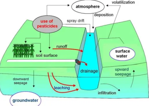
(14) RIVM Report 607407003. 1. Introduction. 1.1. Aim and background of the study As part of the Dutch authorisation procedure for plant protection products (PPPs), an assessment of exposure of aquatic organisms in surface waters adjacent to agricultural fields is required. Spray drift, drainage and runoff are the most important processes involved in loading of edge-of-field surface waters with PPPs (Figure 1). In the evaluation of active substances at the EU level, the importance of all these entry routes is acknowledged (FOCUS 2001). In the current Dutch authorisation procedure, however, spray drift is the only pathway for substances entering the surface water (Beltman and Adriaanse1999, Ctgb 2010). In view of EU-harmonisation, the responsible Dutch Ministries therefore requested the development of a state-of-the-art methodology to also assess the input of PPPs through drainage. This new methodology will become part of a new exposure scenario, which is currently being developed (Tiktak et al. 2012b).. Figure 1 Main processes involved in loading of edge-of-field surface waters with plant protection products. The aims of the study reported here are (i) to adapt the current exposure model PEARL in such a way that it is capable of describing the relevant leaching concentration sufficiently well, and (ii) to parameterise this exposure model for realistic worst-case conditions. Realistic worst-case conditions are generally defined as a combination of soil and climate properties within a certain region for which the predicted environmental concentration (PEC) is equal to a certain percentile of the distribution of concentrations for all climate and soil properties within a region (EFSA 2010). The exact definition of the term ‘realistic worst case conditions’ in the context of the drainpipe exposure scenario is given in Section 1.2.. Page 13 of 106.

(15) RIVM Report 607407003. 1.2. Endpoint of the drainpipe exposure assessment. 1.2.1. Risk management decisions The derivation of the exposure scenario starts with the definition of the endpoint of the exposure assessment. The responsible Dutch ministries decided that the endpoint of the exposure assessment of aquatic organisms should be the 90th percentile of the concentration in Dutch ditches. The ministries additionally decided that the population should be limited to those ditches that will potentially receive both a spray drift load and a drainpipe load of a substance. Figure 2a gives a schematic representation of this population of ditches. The representation shows that this population may be a small subpopulation of the total population of ditches in the Netherlands. See Tiktak et al. (2012b) for further details. In the Netherlands, ditches are classified into four groups, i.e. small or temporarily dry ditches (‘tertiary ditches’), ditches smaller than 3 m (‘secondary ditches’), ditches with a width of 3-6 m at water level (‘primary ditches’), and ditches with a width greater than 6 m. All these ditch types may be edge-of-field ditches. The ministries decided that all these ditch types – also the temporarily dry ditches – should be included in the population of ditches. The work group additionally decided to exclude the ditches with a width greater than 6 m because only 8 per cent of the ditches are in this width class.. Wind direction. A. B. Direction of drains. Potential PPP input from drainpipe Potential PPP input from drift deposition Not included in population of ditches. Not treated with PPP Potentially treated with PPP. Included in population of ditches. Figure 2 Schematic representation of the population of Dutch ditches to be considered in the estimation of the percentile of the concentration of PPP in the surface water. The left-hand panel (A) shows the population to be considered if the selection is based on both drift and drain input. The right-hand panel (B) shows the population to be considered if only drain input is considered. The dashed lines indicate drains.. Page 14 of 106.

(16) RIVM Report 607407003. 1.2.2. Interpretation of the endpoint of the exposure assessment by the working group The working group decided that the drainpipe exposure scenario should apply to the 90th percentile of all ditches that potentially receive PPPs from drainpipes (Figure 2b). In the drainpipe scenario, wind direction is not part of the selection criterion. The implicit assumption is that there is no relationship between wind direction and orientation of ditches, so that it is not possible to exclude ditches based on dominant wind direction. Figure 3 shows that a large proportion of Dutch arable land (40 per cent) has a pipe drainage system.. Figure 3 Presence of a pipe drainage system in the Netherlands (Kroon et al. 2001). The 90th percentile of the exposure concentration applies to ditches in the blue area. The working group further decided that in view of the available time only one drainpipe scenario will be developed. This single scenario should apply to the entire area of arable land. Grassland was excluded from the population of ditches, because PPP-use in grassland is small compared to PPP-use in arable land. In earlier authorisation procedures (Van der Linden et al. 2004), percentiles were based on the area that is potentially treated with the actual PPP for which a notifier requests an authorisation. Application of this procedure would, however, imply that multiple scenarios need to be developed. Due to the non-linearity of the relation between soil parameters, PPP parameters and predicted environmental concentrations, the ranking of scenarios may be different for different ecotoxicologically relevant concentrations. A scenario that is conservative for the peak concentration in water may therefore not be conservative for a time weighted average concentration in water. Moreover, such a scenario is probably not conservative for the PPP-concentration in sediment as well. Nevertheless, the working group decided that the 90th percentile should be based on the annual peak concentration in water. The choice for the peak concentration was based on guidance provided by the ELINK Page 15 of 106.

(17) RIVM Report 607407003. workshop (Brock et al. 2009). The ELINK report states that an effect assessment based on acute toxicity data should always be compared with the peak concentration, whilst in chronic risk assessments in the first instance the peak concentration and under certain conditions a time weighted average concentration may be used. The choice for the peak concentration in water implies that the selected scenarios cannot be used for assessment of concentrations in sediment. In view of the effect of application time on drainpipe concentration, the workgroup decided that the exposure assessment should be carried out for a long-term period, so multiple annual peak concentrations were obtained for each scenario. The workgroup decided that all annual peak concentrations should be used independently, which implies that there is no distinction between space and time. For example 100 ditches and 15 years give 1500 annual maximum concentrations and the target is the 90th percentile of all 1500 values. 1.3. Structure of report Chapter 2 gives an overview of the procedures applied in this report. Chapter 3 gives a description of the preferential flow concepts in PEARL and GeoPEARL. This new conceptual model is applied to the Andelst experimental field site. A description of this application is given in Chapter 4. Chapter 5 describes how additional weather data and groundwater observation data were used to build the exposure scenario. In Chapter 6, we describe the parameterisation and the application of the GeoPEARL model. Chapter 7 describes the derivation of the target temporal percentile to be used in the exposure assessment. Finally, Chapter 8 provides conclusions and recommendations for further developments.. Page 16 of 106.

(18) RIVM Report 607407003. 2. Overview of procedures. The endpoint of the drainpipe exposure assessment is the 90th percentile of the annual maximum concentration in all ditches that potentially receive PPPs from drainpipes. This definition implies that the peak concentration must be known for the entire population of ditches and for multiple years. Spatially distributed PPP-fate models can be used to generate maps of the exposure concentration for the entire area of interest. If an appropriate exposure model exists, the scenario where the 90th percentile peak concentration occurs can be selected directly from the overall distribution function of the so-obtained maps (EFSA 2010). So the first step is to derive an appropriate exposure model. In the Netherlands, the GeoPEARL model (Tiktak et al. 2002, 2003) is the default model for evaluating the leaching of PPPs at the national scale. The model simulates leaching towards drainpipes as well. The current version of GeoPEARL cannot describe the peak concentration in the drainpipe sufficiently well, because this peak concentration is primarily affected by rapid drainage mechanisms due to preferential flow through macropores. For this reason, we developed a new version of (Geo)PEARL, which includes a description of preferential flow. Figure 4 shows the main flow pathways included in this new version. Theoretical backgrounds of the new model are given in Chapter 3. Main flow pathw ays in a macroporous soil column. 1. Soil column Groundwater table. 2. 4 3. Network of cracks. 5. Surface water. 3. Slow drainage tow ards the ditch due to matrix flow. 1. Hortonian and saturation excess runoff. 4. Slow drainage through drainpipes due to matrix flow. 2. Rapid drainage through drainpipes due to macropore flow. 5. Leaching into the regional groundwater. Figure 4 Main flow pathways in a typical Dutch macro-porous soil. The version of GeoPEARL described in Tiktak et al. (2002, 2003) did not include pathway 2. GeoPEARL describes the concentration of PPPs in the drainpipe, but we need the concentration in the ditch. In the exposure scenario, the concentration in ditch water is simulated with the TOXSWA model (Adriaanse 1996). A regional-scale version of TOXSWA is not (yet) available, so we developed a metamodel of TOXSWA, which describes the dilution of the drainpipe concentration in the ditch Page 17 of 106.

(19) RIVM Report 607407003. using a single dilution factor. This factor is a function of the volume of the ditch at the start of the day, the daily volume of drain flow from the upstream catchment and the daily volume of drain flow from the adjacent field. Details of this metamodel are described in Section 3.5. The most straightforward way to obtain the exposure scenario would be by selecting one of the GeoPEARL map-units (also called plots) and base the exposure assessment directly on simulations for this single map unit. We considered this approach as not appropriate, because the lower boundary condition of the GeoPEARL model is extremely simplified: it consists of a longterm average soil water flux on which a sine-function with a fixed amplitude is imposed (Kroon et al. 2001). Because the substance concentration in drain water cannot be simulated sufficiently well with this simplified boundary condition, we decided to use the GeoPEARL simulations only to calculate the relative vulnerability and to base the new drainpipe exposure scenario on a real site instead of on one of the GeoPEARL map-units. The site chosen was the Andelst experimental field site described in Scorza Júnior et al. (2004). At this site sufficient data is available to parameterise and test the PEARL model. The advantage of taking a real site is that full benefit could be taken from the experimental data, so that a consistent and credible exposure scenario could be built. Details on the experimental site are given in Chapter 4. The Andelst dataset covers a period of approximately one year, but the exposure assessment must be carried out for a multi-year period. The dataset was therefore extended to a 15-year period using data from a weather station at a distance of 40 km and a nearby groundwater observation point (the length of the dataset was 15 years and not 20 years as in GeoPEARL because the groundwater observation dataset had a length of 15 years). Consequently, the exposure assessment results in 15 annual peak concentrations. GeoPEARL was used to determine which of these annual peak concentrations corresponds to the 90th percentile of the exposure concentration in all ditches. This was done as follows: 1. GeoPEARL was run for a 20-year period, so 20 annual peak concentrations were obtained for each map unit; 2. A cumulative distribution function (cdf) of all annual peak concentrations was constructed in which each peak concentration was given a weight proportional to the total ditch length associated with the corresponding GeoPEARL plot, and the 90th percentile was calculated from this overall cdf (red line in Figure 5); 3. For the Andelst scenario, a cumulative distribution function of the 15 annual maximum concentrations was created (green line in Figure 5); 4. The target temporal percentile is the temporal percentile that predicts the same concentration as the 90th percentile of the overall cdf. This percentile can be looked up by following the arrows A, B and C in Figure 5. In our example, the target temporal percentile to be used in the exposure assessment is 20 per cent. Further details on the derivation of the target percentiles are given in Chapter 7.. Page 18 of 106.

(20) RIVM Report 607407003. Figure 5 Procedure to derive the target temporal percentile to be used in the exposure assessment. For the Andelst scenario, the target temporal percentile predicts the same concentration as the 90th percentile of the overall cumulative distribution function (red line). The selected temporal percentile should be sufficiently conservative for all relevant substances. However, due to the non-linearity of the relation between soil parameters, PPP-fate parameters and predicted environmental concentrations, the ranking of climate and soil property combinations is different for different substance properties. As a consequence, a temporal percentile derived for one substance may not be sufficiently conservative when applied to another substance. To overcome this problem, the target temporal percentile was calculated for multiple substances with different degradation half-lives and sorption coefficients. Based on these two properties, the software tool DRAINBOW will automatically select the target temporal percentile to be used in the exposure assessment. The above procedure differs in two fundamental ways from the scenario selection procedure that was recently published by EFSA (2010). EFSA (2010) proposes selecting an exposure scenario using a (simplified) spatially distributed model and then parameterising this scenario. In our procedure, we have reversed this order: we parameterise an exposure scenario using data from an existing field site and then put the simulations into context using results from a spatially distributed model. This was done because we wanted to benefit from the monitoring data available at the field site. The second difference is that we did not consider uncertainty during the scenario development. Van den Berg et al. (2008), Heuvelink et al. (2010) and Vanderborght et al. (2011) showed that the 90th percentile of the leaching concentration of PPPs generally shifts towards higher values if uncertainty of PPP-properties and scenario properties is considered. Because ignoring uncertainty may lead to scenarios that are not sufficiently conservative, EFSA (2010) recommends already taking uncertainty into account when developing new scenarios. An uncertainty analysis with the newly developed GeoPEARL model is, however, not yet available. Page 19 of 106.


(22) RIVM Report 607407003. 3. Macropore concepts in (Geo)PEARL. 3.1. Introduction PEARL and GeoPEARL are now commonly used in PPP authorisation procedures and policy evaluations. For example, in the Netherlands the GeoPEARL model (Tiktak et al. 2002, 2003) is used to evaluate the leaching to the groundwater (Van der Linden et al. 2004). In surface waters, the peak concentration is considered an important exposure endpoint. This endpoint is mainly determined by the peak concentrations in the drainpipe. So far, PEARL has been less suitable to describe this peak concentration, because it is primarily affected by rapid drainage mechanisms and surface overland flow. For this reason, macropore versions of PEARL and GeoPEARL have been developed. The macropore versions of the two models play a crucial role in the new exposure scenario. The macropore version of PEARL is based on FOCUS PEARL_3_3_3, which is described in Leistra et al. (2000), Tiktak et al. (2000) and Van den Berg et al. (2006). PEARL is a one-dimensional, multi-layer model, which describes the fate of a PPP and its transformation products in the soil-plant system. The model is linked with the Soil Water Atmosphere Plant (SWAP version 3.2) model (Kroes et al. 2008). The macropore version of PEARL describes the transport of PPPs through the soil matrix and through two preferential flow domains, i.e. a bypass domain and an internal catchment domain (Kroes et al. 2008). Macropores can be either permanent or temporary (due to shrinking of soils). The feature of describing swell and shrink characteristics of soils was considered important, because Dutch clayey soils generally have a high content of vermiculites and smectites (Breeuwsma 1985, Breeuwsma et al. 1986, Van der Salm 2001). Soils with these clay minerals have a large shrink and swell potential (Scheffer et al. 1979, Bronswijk and Evers-Vermeer 1990).. 3.1.1. Dominant flow paths The Netherlands is situated in a relatively flat delta area, characterised by shallow groundwater tables and a high density of the drainage network. Description of the interaction between soil water, regional groundwater and surface water is indispensable in lowland areas (Figure 4). Surface overland flow (in PPP modelling often called ‘runoff’) can occur if the infiltration capacity is exceeded in (fine-textured) soils (Horton 1940). When macropores are present, overland flow may be routed into macropores at the soil surface. Parts of these macropores penetrate deeply into the soil and are horizontally connected. Water routed into these macropores bypasses the reactive unsaturated soil, leading to rapid drainage towards drainpipes and short circuiting between the soil surface and the groundwater. A part of the macropores ends at various depths in the unsaturated zone, forcing macropore water to infiltrate in the soil matrix at a larger depth (Van Stiphout et al. 1987). Under wet conditions, however, soils may be swollen so that macropores are closed. In this case, overland flow may be routed directly into surface waters. The importance of surface overland flow in lowland areas was confirmed in recent studies in the Netherlands (Rozemeijer and Van der Velde 2008, Rozemeijer et al. 2010, van der Velde et al. 2010) and Illinois (Algoazany 2007). In regions with shallow groundwater tables, overland flow may also occur when the soil profile is completely saturated. This process – called saturation excess overland flow – may occur after light rainfall of long duration. In coarsely textured soils, matrix flow is the dominant process. Page 21 of 106.

(23) RIVM Report 607407003. 3.1.2. Chapter overview This chapter describes the theory behind the macropore version of PEARL. In this report, only those processes are described which are relevant for understanding the parameterisation of the new drainpipe exposure scenario. Section 3.2 describes the mathematical description of macropore geometry in SWAP. Section 3.3 gives a short overview of the hydrological concepts conceived in SWAP. A more comprehensive description of macropore concepts in SWAP can be found in Kroes et al. (2008). Section 3.4 gives a description of the PPP transport routines. PEARL calculates the concentration in drain water, but we need the concentration in ditch water. In the exposure scenario, this concentration is simulated with the TOXSWA model (Adriaanse 1996). In the scenario selection phase, we used a simple metamodel of TOXSWA, which is described in Section 3.5.. 3.2. Macropore geometry. 3.2.1. Conceptual model In SWAP, macropore geometry is described on the basis of three properties, i.e. continuity, persistency and macropore shape. Continuity Macropores are divided into two domains (Figure 6): • The main bypass flow domain, which is a network of continuous, horizontally interconnected macropores. These macropores penetrate deep into the soil profile and are assumed to be horizontally interconnected. In the main bypass domain, water is transported fast and deep into the soil profile, bypassing the soil matrix. This may lead to rapid drainage towards drainpipes and short-circuiting between the soil surface and the groundwater. • The internal catchment domain, which consists of discontinuous, noninterconnected macropores ending at different depths in the profile. In this domain, water is captured at the bottom of individual macropores, resulting in forced infiltration of macropore water into the soil matrix. Persistency The macropore volume of the two domains is further subdivided into a static macropore volume and a dynamic macropore volume. The static macropore volume consists of structural shrinkage cracks, bio-pores and macropores that originate from tillage operations. Dynamic macropores originate from the shrinking of the soil matrix due to soil moisture loss. Shrinking is generally restricted to soils that contain a substantial amount of interlayered clay minerals (particularly smectites and vermiculites) and/or organic matter (peats). Macropore shape Macropore shape is described by an effective soil matrix polygon diameter (dpol). Macropore shape affects the exchange of water between the soil matrix and the macropores: in soils with a large effective matrix polygon diameter, exchange will be relatively slow because of the relatively small vertical area of macropore walls per unit of horizontal area. The effective matrix polygon diameter is also related to crack width, which affects rapid drainage to drainpipes. It is assumed that the effective soil matrix polygon diameter is a function of depth with its minimum value at the soil surface where macropore density is maximal, and consequently distances between macropores are relatively small. Page 22 of 106.

(24) RIVM Report 607407003. Figure 6 Schematic representation of the two macropore domains, i.e. the main bypass domain transports water deep into the soil profile possibly leading to rapid drainage and the internal catchment domain in which infiltrated water is trapped into the unsaturated soil matrix at different depths. The black lines represent the schematic representation of the macropore volume as depicted in Figure 7. 3.2.2. Mathematical model SWAP offers a large number of options to describe macropore geometry (Kroes et al., 2008). In PEARL, only those options are implemented for which parameters can be found through pedotransfer functions (see Chapter 6). Depth distribution of macropores In PEARL, the volume fraction of static macropores in the two domains as a function of depth (Vsta,z (m3 m-3)) is described by a stepwise linear function (denoted by the solid line in Figure 7):. V= Vsta,byp,0 + Vsta,ica,0 sta, z. for.  z −z  V= Vsta,byp,0 − Vsta,ica,0  Ah  for sta, z  z Ah − zica   z −z  V= Vsta,byp,0 − Vsta,byp,0  ica sta, z  for  zica − zsta . 0 ≥ z > z Ah z Ah ≥ z > zica zica ≥ z > zsta. (1). where Vsta,byp,0 (m3 m-3) is the volume fraction of the static macropores in the bypass domain at soil surface, Vsta,ica,0 (m3 m-3) is the volume fraction of static macropores in the internal catchment domain at soil surface, zAh (m) is the depth of the plough layer, zica (m) is the bottom depth of the internal catchment domain, and zsta (m) is the bottom depth of the static macropore domain. In PEARL, the user has to input the total volume fraction of static macropores at soil surface and the volumetric proportion of the internal catchment domain with respect to the static macropores at the soil surface, Pica, 0 (-): = Pica,0. Vsta,0,ica Vsta,0,ica = Vsta,0 Vsta,0,ica + Vsta,0,byp. (2). Page 23 of 106.

(25) RIVM Report 607407003. Pica,0 determines the distribution over the two main domains of the precipitation water routed into the macropores at soil surface.. Figure 7 Mathematical representation of the static macropore volume as a function of depth. zah (m) is the depth of the plough layer, zIca (m) is the bottom depth of the internal catchment domain, zsta (m) is the bottom depth of the permanent macropores, VSta,byp,0 (m3 m-3) is the volume fraction of macropores in the bypass domain, and VSta,Ica,0 (m3 m-3) is the volume fraction of macropores in the internal catchment domain. Dynamic macropores due to soil shrinkage Besides static macropores, also dynamic macropores (due to soil shrinkage) may be present. The volume fraction of dynamic macropores is added to the volume fraction of the static macropores (Figure 7). The constant Pica,0 (Equation 2) is used to distribute the total macropore volume over the two macropore domains, so for static and dynamic alike. See Kroes et al. (2008) for details. Notice that due to shrinkage, macropores can be temporarily present at greater depths than zsta in Figure 7. The increase of the volume of dynamic macropores is equal to the volume of horizontal shrinkage of the soil matrix. For the relation between horizontal and total shrinkage of the soil matrix isotropic shrinkage is assumed. Total shrinkage is measured by drying soil aggregates (Bronswijk and EversVermeer 1990). For each soil, there is a fixed relationship between moisture content and the volume of the soil matrix (the shrinkage characteristic). Figure 8 shows a typical example of a shrinkage relationship of a clay soil. Three stages of shrinkage can be distinguished (Scheffer et al. 1979; Bronswijk and EversVermeer 1990), i.e. normal shrinkage (volume loss of aggregates is equal to moisture loss), residual shrinkage (volume loss of aggregates is less than moisture loss) and zero shrinkage (soil particles have reached their densest configuration). Description of the shrinkage characteristic requires two userspecified parameters, i.e. the void ratio at moisture ratio zero (oven dry water content) and the moisture ratio at transition of residual to normal shrinkage. The void ratio and the moisture ratio are defined as:. Page 24 of 106.

(26) RIVM Report 607407003. e=. φ =. Vp. (3). Vsoil. θ. (4). 1 − θs. where e (-) is the void ratio, Vp (m3 m-3) is the volume fraction of pores in the soil matrix, and Vsol (m3 m-3) is the volume fraction of the solid soil, φ (-) is the moisture ratio, θ (m3 m-3) is the volume fraction of soil water, and θs (m3 m-3) is the volume fraction of soil water at saturation. The relation between void ratio as function of moisture ratio and shrinkage volume is:. Vshr =. ( e − es ) Vsol. (5). where es is void ratio at saturation. Void ratio (-). Zero shrinkage Residual shrinkage Normal shrinkage e0. φa. Saturation line. Moisture ratio (-). Figure 8 Typical shrinkage characteristic of a clay soil showing the three shrinkage stages. The black dots represent the typical points that have to be specified by the user, i.e. the void ratio at zero moisture content e0 (-) and the moisture ratio at transition from normal to residual shrinkage φa (-). Effective diameter of soil polygons The effective diameter of the soil polygons is assumed to be a function of depth with its minimum value at soil surface where macropore density is highest and consequently distances between macropores are small, and its maximum value deeper in the soil profile:.   V dpol , z =dpol ,min + (dpol ,max − dpol ,min ) 1 − sta, z   Vsta,0  . (6). Where dpol,min (m) is the minimum polygon diameter, dpol,max (m) is the maximum polygon diameter, Vsta (m3 m-3) is the volume fraction of static macropores (m3 m-3), and Vsta,0 (m3 m-3) is the volume fraction of static macropores at soil surface.. Page 25 of 106.

(27) RIVM Report 607407003. 3.3. Water flow SWAP simulates the water balance of the bypass domain and the internal catchment domain separately:. dWbyp dt. = I p,byp + Ir ,byp −. z zgwl z zgwl ,byp = z= =0. ∫. zgwl. ∫. Rlu,bypdz −. zsta. Rls,bypdz −. ∫. zsta. Rd ,bypdz. (7). With. dWica = I p,ica + Ir ,ica − dt. z =0. ∫. zgwl. Rlu,icadz −. z = zgwl. ∫. zica. Rls,icadz. (8). where suffix byp refers to the bypass domain, suffix ica is the internal catchment domain, W (m3 m-2) is the areic volume of water in the macropores, t (d) is time, Ip (m3 m-2 d-1) is the areic volume rate of infiltration of water at soil surface by direct precipitation, Ir (m3 m-2 d-1) is the areic volume rate of infiltration through runoff, Rlu (m3 m-2 d-1) is the volumic volume rate of lateral infiltration into the unsaturated matrix, Rls (m3 m-2 d-1) is the volumic volume rate of lateral flow into and out of the saturated soil matrix, Rd (m3 m-2 d-1) is volumic volume rate of drainage, z is the depth, zgwl is the depth of the groundwater table, and zgwl,byp (m) is the depth of the water table in the bypass domain. All balance terms are positive, except Rls which is positive in case of flow into the matrix and negative in the case of flow out of the matrix, and Rd which is positive in the case of flow towards the drainage system and negative in the case of flow from the drainage system. Note that the water balance of the internal catchment domain does not contain a drainage term because it is assumed that macropores in this domain end above the drains. Vertical flow in the macropores is calculated from the water balance of the individual soil layers, see Kroes et al. (2008) for details. SWAP can also simulate water flow into macropores by interflow, which may occur if a perched groundwater table is present. This term is not further described here, because it is not used within PEARL. Inflow at soil surface The rate of precipitation and irrigation water routed directly into the macropores at soil surface is calculated as: I p,ica = Pica,0 Amac P I p,byp= (1 − Pica,0 )Amac P. (9) (10). where P (m3 m-3 d-1) is the sum of precipitation, irrigation rate and snowmelt, Pica,0 (-) is the proportion of the internal catchment domain at soil surface (Eqn. 2), and Amac (m2 m-2) is the horizontal macropore volume fraction at soil surface, which is assumed to be equal to the total macropore volume at soil surface, Vmac,0. Runoff into macropores occurs when the total rate of precipitation, irrigation and snowmelt exceeds the infiltration capacity of the soil matrix (Hortonian overland flow). In this case, ponding occurs, and the infiltration rate is calculated as: Ir =. h0 γr. Page 26 of 106. (11).

(28) RIVM Report 607407003. where h0 (m) is the ponding depth and γr (d) is the resistance for macropore inflow at soil surface. In surface runoff calculations, usually a threshold ponding depth is used before runoff starts. This is not the case in the calculation of runoff into macropores, because it is assumed that micro depressions are connected to macropores. It can further be shown (Bouma and Anderson 1973) that infiltration resistances are low (0.01-0.001 d). The effect of both assumptions is that ponding water is routed preferentially into the macropores. Distribution of Ir over the bypass domain (Ir,byp) and the internal catchment domain (Ir,ica) is according to their volumetric proportions at soil surface, Pbyp,0 and Pica,0. Runoff from the field directly into the adjacent ditch occurs only if the macropores are fully saturated. Lateral infiltration into the unsaturated matrix Lateral infiltration of macropore water into the unsaturated soil matrix occurs over the depth where macropore water is in contact with the unsaturated matrix. In PEARL, it is assumed that absorption is the dominate process. Absorption is described with Philip’s sorptivity (Philip 1957): Rlu =. 4S(θ)p t − t0. (12). dpol 1 − Vmac. Where Rlu (m3 m-3 d-1) is the volumic volume rate of absorption over time interval t0 → t (d), and S(θ)p (m3 m-2 d0.5) is Philip’s sorptivity. Philip’s sorptivity depends on the initial water content. Lateral infiltration into and exfiltration out of the saturated matrix Lateral infiltration of macropore water into the saturated soil matrix occurs over the depth where macropore water is in contact with the saturated matrix. Lateral infiltration and exfiltration is calculated with a Darcy equation (Eqn. 13): Rls =. fshp 8K s (hmac − hmic ). (13). 2 dpol. where Rls (m3 m-3 d-1) is the volumic volume rate of infiltration, and K (m d-1) is the saturated hydraulic conductivity of the soil matrix, hmac (m) is the hydraulic head in the macropore, and hmic (m) is the hydraulic head in the micropore domain. Parameter fshp (-) is a shape factor, which accounts for uncertainties in the theoretical description of lateral infiltration by Darcy flow originating from uncertainties in the exact shape of soil matrix polygons. In PEARL, a default value of 1 is used (Kroes et al. 2008). Note that infiltration occurs if hmac > hmic and exfiltration occurs if hmac < hmic. Rapid drainage Rapid drainage to drainage systems may occur via a network of horizontally interconnected macropores. In SWAP, rapid drainage is calculated using a drainage resistance: qrd =. zgwl ,byp − zdra γ rd ,act. (14). where qrd (m3 m-2 d-1) is the rapid drainage flux, zgwl,byp (m) is the water level in the bypass domain, zdra (m) is the depth of the pipe drainage system, and γrd,act (d) is the actual rapid drainage resistance. The drainage resistance decreases with increasing groundwater level, and is calculated from the reference drainage Page 27 of 106.

(29) RIVM Report 607407003. resistance and the ratio between the actual and reference transmissivity [KD] of the macropores: γ= act. [KD]act γ [KD]ref ref. (15). where. = [KD]. zgwlbyp. zgwlbyp. zsta. zsta. = ∫ Klat d z C. ∫. wmp dpol. dz. (16). in which Klat (m d-1) is the lateral hydraulic conductivity of the macropores, zsta (m) is the bottom depth of the bypass domain when reaching into the saturated soil, zgwlbyp (m) is the depth of the water level in this domain, and wmp (m) is the macropore width. The value of C is a hypothetical constant, which is not relevant because it is eliminated in Eqn. 15. The volumic volume rate of rapid drainage in Eqn 7 is calculated by distributing the rapid drainage flux over the water filled soil layer (i.e. the layer from zsta to zgwl,byp) according to the relative transmissivity of the macropores in the bypass domain:. Rd ,byp =. [KD] z = zgwl ,byp. ∫. qrd. (17). [KD]dz. zsta. 3.4. Substance behaviour Substance balance Substances in the macropore domain are assumed to reside in a water layer at the bottom of the two macropore domains (Figure 6). The major pathway for substances entering the macropores is surface runoff. Substances can also enter the macropores by exfiltration out of the saturated soil matrix. Notice, however, that this process can only occur in static macropores, because the volume fraction of dynamic macropores is zero in saturated soils due to swelling. In the internal catchment domain, infiltration from the macropores into the saturated or unsaturated soil is the only loss process. In the bypass domain, rapid drainage is an additional loss term, possibly leading to direct surface water contamination. It is further assumed that degradation in the macropore domain is zero. This is justified, because of the short residence times in the macropores. The substance balances of the two macropore domains read: = z 0= z 0 dAica = Jr ,icadz + ∫ Je,icadz ∫ dt zmix zsta. (18). z 0= z 0= z 0 = dAbyp = Jr ,bypdz + Je,bypdz + Jd ,bypdz dt zmix zsta zsta. ∫. ∫. ∫. (19). where Aica (kg m-2) is the areic mass of substance in the macropore system, Jr (kg m-3 d-1) is the volumic mass rate of substance runoff into the macropores, Je (kg m-3 d-1) is the volumic mass rate of exchange between the soil matrix and the macropore system, and Jd (kg m-3 d-1) is the lateral volumic discharge rate of substance due to rapid drainage. All balance terms are positive, except for Re, which is negative when substance flow is from the macropores into the matrix. Page 28 of 106.

(30) RIVM Report 607407003. The suffixes ica and byp refer to internal catchment domain and bypass domain, respectively. The variable zmix (m), the mixing layer depth, is explained in the following paragraph. The areic mass of substance is calculated as: Aica = WicacL,ica. (20). A= WbypcL,byp + fs,bypξbyp X byp byp. (21). where W (m3 m-2) is the areic volume of water in the macropore (i.e. the water layer), cL (kg m-3) is the substance concentration in the macropore, fs,byp (-) is the fraction of solid phase in contact with the bypass domain, ξbyp (kg m-2) is the areic mass of solid phase in soil over the water-filled depth of the bypass domain, and Xbyp (kg kg-1) is the mass of substance sorbed per mass of dry soil in the bypass domain. So ξbyp is defined as zwet , byp,end. ζ= byp. ∫. (22). ρ dz. zwet , byp, start. where zwet,byp,start (m) is the depth where the wet part of the bypass domain starts and zwet,byp,end (m) is the depth where the wet part of the bypass domain ends. For the bypass domain only Freundlich equilibrium sorption is assumed. The Freundlich coefficient, KF,byp is described by (23). K F ,byp = OMbypKOM. where OMbyp (kg kg-1) is average organic matter over the depth of the waterfilled bypass domain. From Eqn 21, the expression of the substance concentration in the bypass domain, c*byp, can be derived by dividing all terms by Zwet,byp, i.e. the thickness of the wet part of the bypass domain. This gives: * cbyp = θbypcL,byp + fs,bypρbyp X byp. (24). where θbyp is the volume fraction of water of the bypass domain and ρbyp is the average dry bulk density over the depth of the water-filled bypass domain. Please note that Eqn. 24 is only needed for calculating the distribution over solid and liquid phase within the bypass domain. Mass conservation is ensured by Eqn. 21. The substance balance of the soil matrix is extended as follows:. ∂c *eq ∂t. = − Js −. ∂Jp,L ∂z. −. ∂Jg,L ∂z. − Jt + Jf − Ju − Jd − Je. (25). Here, c*eq (kg m-3) is the substance concentration in the equilibrium domain of the soil system, Js (kg m-3 d-1) is the volumic mass rate of substance sorption in the non-equilibrium domain, Jp,L (kg m-2 d-1) is the mass flux of substance in the liquid phase, Jp,g (kg m-2 d-1) is the mass flux of substance in the gas phase, Jt (kg m-3 d-1) is the transformation rate, Jf (kg m-3 d-1) is the formation rate, Ju (kg m-3 d-1) is the rate of substance uptake by plant roots, Jd (kg m-3 d-1) is the lateral discharge rate of substances, and Je (kg m-3 d-1) is the lateral exchange rate between the matrix and the macropore domain (negative if Page 29 of 106.

(31) RIVM Report 607407003. substance flow is from the macropore domain into the matrix). The substance balance of the non-equilibrium domain is not affected. Input of substance by surface runoff Surface overland flow is the main pathway for substances entering the macropores. PEARL uses a mixing layer concept to describe the interaction between surface runoff and the top soil layer. In this concept, it is assumed that chemicals are released from a thin layer of topsoil that interacts with rainfall and runoff (Ahuja et al. 1982, Sharpley 1985). Sharpley (1985) reviewed several runoff studies and found mixing layer depths between 0.13 and 3.7 cm. They also found that the ‘effective depth of interaction’ increased with rainfall intensity and slope (i.e. with runoff energy) and decreased with increasing soil aggregation. Because data are lacking to parameterise these relationships, PEARL uses a constant mixing layer depth, zmix. In PEARL, the first numerical soil compartment acts as the mixing layer. The mass balance for the first compartment is extended with a runoff term:. ∂c *eq ∂t. = − Js −. ∂Jp,L ∂z. −. ∂Jg,L ∂z. − Jt + Jf − Ju − Jd − Je − Jr. (26). where Jr (kg m-3 d-1) volumic mass rate of substance discharge in runoff. Jr consists of three terms, i.e. runoff into the bypass domain (Jr,byp), runoff into the internal catchment domain (Jr,ica) and runoff from the field (Jr,fld). These terms are calculated as follows: Jr ,byp = (fmix Ir ,bypcL,mix ) / zmix. (27). Jr ,ica = (fmix Ir ,icacL,mix ) / zmix. (28). Jr ,fld = (fmix Ir ,fld cL,mix ) / zmix. (29). Parameter fmix (-) is the runoff extraction ratio. This parameter is a lumped parameter that accounts for physical non-equilibrium between the soil and runoff (Gouy et al. 1999). Physical non-equilibrium results, among others, from water flow on the soil surface, which is not homogeneous. Exchange between the soil matrix and the macropores Convection is the only process considered in the exchange between macropores and the soil matrix: = Je,byp Re,bypcL,byp. if. Re,byp ≤ 0. = Je,byp Re,bypcL,mic. if. Re,byp > 0. = Je,ica Re,icacL,ica. if. Re,ica ≤ 0. = Je,ica Re,icacL,mic. if. Re,ica > 0. (30). (31). where cL,mic (kg m-3) is the substance concentration in the liquid phase of the micropore domain, cL,byp (kg m-3) is the substance concentration in the bypass domain and cL,ica (kg m-3) is the substance concentration in the internal catchment domain. The volumic volume rate of exchange between the macropore and the soil matrix, Re,byp or Re,ica, is equal to the lateral infiltration into or exfiltration out of the saturated matrix (Rls) in the saturated zone, and equal to volumic volume rate of infiltration Rlu in the unsaturated zone. Page 30 of 106.

(32) RIVM Report 607407003. Substance discharge by drainage PEARL calculates rapid drainage from the bypass domain as well as lateral discharge through the soil matrix (Section 3.1). Lateral discharge of substances by drainage is taken proportional to the volumic volume rates of water: Jd ,byp. Rd ,bypcL,byp. Jd ,byp. 0. Jd ,mic. Rd ,mic cL,mic. Jd ,mic. 0. if if if if. Rd ,byp > 0. (32). Rd ,byp ≤ 0 Rd ,mic > 0. (33). Rd ,mic ≤ 0. where Jd,byp (kg m-3 d-1) is the volumic mass rate of substance discharge in rapid drainage, Jd,mic (kg m-3 d-1) is the volumic mass rate of substance discharge from the soil matrix, Rd,byp (m3 m-3 d-1) is the volumic volume rate of rapid drainage, and Rd,mic (m3 m-3 d-1) is the volumic volume rate of drainage from the soil matrix. Eqn. 32 and 33 imply that it is assumed that concentration gradients in the lateral direction are negligible (i.e. no diffusion and dispersion). The concentration in drainage water, cL,d, is calculated using flux-weighted averaging procedure:. cL,d =. 3.5. ∞. ∞. 0 ∞. 0 ∞. 0. 0. ∫ Jd,micdz + ∫ Jd,bypdz. (34). ∫ Rd,micdz + ∫ Rd,bypdz. The peak concentration in ditch water PEARL describes the concentration of substances in drain water, but we need the concentration in the ditch. In the final exposure scenario, substance fate in ditch water is simulated with the TOXSWA model (Adriaanse, 1996). In the scenario selection phase, we need a regional-scale substance fate model, because we need the peak concentrations for the entire population of Dutch ditches (Section 1.2). A regional-scale version of TOXSWA is, however, not (yet) available. For this reason, Adriaanse (personal communication, 2009) created a metamodel of TOXSWA, which calculates the dilution of the drainpipe concentration based on the volume of the ditch at the start of the day, the daily volume of drain flow from the upstream catchment and the daily volume of drain flow from the adjacent field:. cditch = e −αB. Vadj Vditch. cL ,d + (1 − e −αB ). Vadj + f upstr .treatedVupstr ,total Vadj + Vupstr ,total. c L ,d (35). where cditch (μg/l) is the concentration in ditch water, Vadj (m3 m-1) is the lineic volume 1 of daily drain flow from the adjacent field, Vditch (m3 m-1) is the lineic volume of the ditch at the start of the day, Vupstr,total (m3 m-1) is the lineic volume of daily drain flow from the upstream catchment, fupstr,treated (-) is the fraction of the upstream catchment that is treated, cL,d (μg/l) is the concentration in drain water calculated with Eqn. 34, α (-) is a calibration factor, and B (-) is equal to:. 1. The volume of water per length. Page 31 of 106.

(33) RIVM Report 607407003. B=. Vadj. Vadj + Vupstr ,total. Vditch Vadj + fupstr ,treatedVupstr ,total. (36). The initial lineic volume of the ditch is calculated with the equation:. Vditch = bh + s1h2. (37). where b (m) is the width at ditch bottom, h (m) is the water depth, and s1 (-) is the slope of the watercourse sides, expressed as the ratio of the horizontal distance and the vertical distance. The daily volume of drain water is calculated with the equations: Vadj =. t +∆t. ∫ t. qd Aadj dt. Vupstr ,total =. t +∆t. ∫ t. qd Aupstr dt. (38). (39). in which Aadj (m2 m-1) is the area of the adjacent field per unit ditch length, Aupstr (m2 m-1) is the area of the upstream catchment per unit ditch length, t (d) is time and qd (m3 m-2 d-1) areic volume flux of drainage from the adjacent field. The implicit assumption is that the drainage flux from the upstream catchment is equal to the drainage flux from the adjacent field. The drainage flux consists of rapid drainage due to flow through the main bypass domain and a slow drainage term due to flow through the soil matrix: = qd qd ,mic + qd ,byp. (40). where qd,mic (m3 m-2 d-1) is the areic volume flux of drainage due to flow through the soil matrix, and qd,byp (m3 m-2 d-1) is the areic volume flux of drainage due to flow through the main bypass domain. The metamodel was calibrated to the FOCUS D3 scenario (FOCUS 2001). The so-obtained value of α was equal to 2. Example results for a range of ditch volumes are shown in Figure 9. It can be seen that the initial concentration in ditch water equals the concentration in drain water at high drainage fluxes. At small initial ditch volumes, a daily drainage flux of 2 mm d-1 is sufficient to completely refresh the water initially present in the ditch.. Page 32 of 106.

(34) RIVM Report 607407003. Figure 9 Initial concentration in ditch water as a function of the drainage flux from the adjacent field. The concentration in the drainpipe was set to 1 μg/L, α was set to 2, and both the area of the adjacent field and the area of the upstream catchment were set to 100 m2 m-1. As a conservative assumption, 100% of the area upstream was assumed to be treated.. Page 33 of 106.


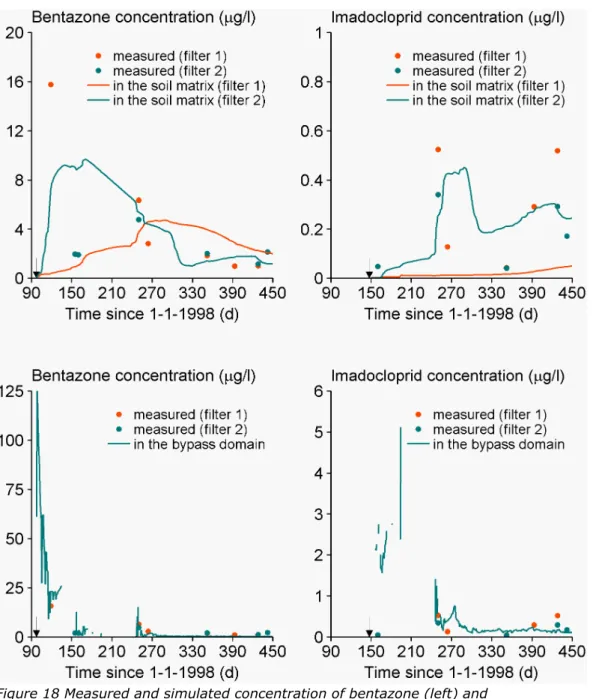
(36) RIVM Report 607407003. 4. Application of the macropore version of PEARL to the Andelst field study. 4.1. Introduction The Andelst field study plays a crucial role in the development of the drainpipe exposure scenario. It is currently the only Dutch dataset where sufficient data is available to parameterise and test all modules of the preferential flow version of PEARL. Other field studies are available for testing parts of the model as well, but they either lack measurements of pesticide fate (Hendriks et al. 1999; Van den Beek et al. 2008) or were carried out in a sandy soil (Boesten and Van der Pas 2002). For this reason, we decided to base the new drainpipe exposure scenario on data obtained from the Andelst experimental field site. This chapter presents the application of PEARL to the Andelst experimental field site. The purpose of the study reported in this chapter was to test the conceptual model described in Chapter 3. Section 4.2 gives a brief introduction to the Andelst dataset. Section 4.3 describes the derivation of the input data. In Section 4.4, results are presented and discussed. Finally, Section 4.5 gives some general conclusions. Chapter 5 will describe the parameterisation of the PEARL drainpipe scenario, based on the experiences gained in this chapter.. 4.2. Field study The experiment was carried out from April 1998 until April 1999 in a field located near the municipality of Andelst (51o 53’N; 5o 43’E; altitude 8 m above sea level) and is described in detail by Smelt et al. (2001) and Scorza Júnior et al. (2004). The experimental field was 160 m long and 50 m wide. The experimental field was drained at a depth of 80 – 90 cm. Drain spacing is 10 m. The experimental field comprised the entire catchment area of six drainpipes. Three adjacent drain outlets were merged into one drain set, hence we have two drain sets. The water table resided at a depth of 60 – 180 cm below the soil surface. The soil is a young Holocene river bank deposit of the river Rhine and is classified as a Eutric Fluvisol (FAO 1988). Table 1 summarises some general soil properties. Notice that the organic matter content was obtained from the organic carbon content and not from ignition loss. Shrinkage cracks were observed at the soil surface. Permanent macropores (for example worm holes) were regularly found in the subsoil (26 – 100 cm soil layer). At a depth of about 3 m, a thick layer of coarse sand underlies the clay profile, which is in direct contact with the river Waal (at 1 km distance), and thus acts as a natural drain. On 23 October 1997 winter wheat was sown, and harvested on 20 August 1998. On 8 December 1998, the field was ploughed (25–30 cm) and winter wheat was sown again. A very mobile chemical (bentazone [3-isopropyl-1 H2,1,3,benzothiadizin-4-(3H)-one 2,2 dioxide]) was applied on 7 April 1998 at a rate of 1.33 kg active ingredient ha-1. Within 12 hours after bentazone application, 6 mm of rain fell, which washed off most of the chemical from the wheat crop. A moderately sorbing, persistent chemical (imidacloprid [1-((6-chloro-3-pyridinyl)-methyl)-N-nitro-2-imidazolidinimine] was applied on 27 May 1998 at a rate of 0.7 kg active ingredient ha-1.. Page 35 of 106.

(37) RIVM Report 607407003. Table 1 Soil properties at the experimental field in Andelst. Values are averages of four samples and percentages are given by mass. Standard deviation is generally less than 10%. Layer Properties (cm) pH-KCl OMa Clay Silt Sand Bulk density (%) (%) (%) (%) (kg m-3) 0–26 7.1 2.1 28 53 19 1466 26–50 7.1 1.1 30 51 19 1508 50–70 7.4 1.0 35 51 14 1520 70–90 7.4 1.0 37 49 14 1504 90–120 7.5 1.0 37 47 16 1620 a). calculated from the organic carbon content (%OM = %OC/0.58), where 0.58 is the average C-content of organic matter (Scheffer et al. 1979).. Rainfall was measured continuously with a tipping bucket device installed at the experimental site. Soil temperatures, phreatic groundwater levels and drain discharge were measured continuously as well. Other meteorological data were obtained from meteorological station ‘De Haarweg’ in Wageningen, situated at 10 km from the experimental site. Soil samples were taken from 16 soil columns (diameter 10 cm) at 1, 22, 52, 69, 125, 167, 239 and 378 days after bentazone application. Sampling was to a depth of 1.2 m. After sampling, the columns were sliced into 10 cm layers, and the concentration of the chemicals in the soil was determined. Soil water content and the dry bulk density were measured as well. A total of 16 groundwater sampling tubes were installed with filters at 1.0 – 1.2 m, 1.3 – 1.5 m and 1.9 - 2.8 m depth. Soil and groundwater samples from corresponding depths were combined to four samples and analysed for bentazone and imidacloprid. Drain water was proportionally sampled in the two drain sets using a cooled ISCO model 3700 R sampler that was attached to an ISCO 3200 flow meter. 4.3. Model parameterisation Where possible, the input parameters were based on direct measurements, expert judgement and pedotransfer functions. Only in those cases where parameters could not be obtained in this way, was calibration carried out. This section describes the first group of parameters, the calibration parameters are described in Section 4.4. Boundary conditions and drainage characteristics The bottom boundary flux was calculated using the hydraulic head difference between the phreatic groundwater and the groundwater in the underlying semiconfined aquifer (Cauchy condition): qbot =. Φ aqf − Φ gwl γ aqt. (41). where Φaqf (m) is the hydraulic head of the semi-confined aquifer, Φgwl (m) is the phreatic head and γaqt (d) is the vertical resistance of the acquitard. Hydraulic heads were available from continuous measurements. The measurements showed that the head gradient was generally small, so the vertical resistance was set to a small value of 5 days.. Page 36 of 106.

(38) RIVM Report 607407003. The drainage base and the drainage resistance were obtained from linear regression between measured drain fluxes and groundwater levels (Ter Horst et al. 2006). They obtained a drainage base of 0.8 m and a drainage resistance of 14 days. The so-obtained drainage resistance was assigned to the rapid drainage system (i.e. the macropores). Because the drainage resistance of the soil system as a whole (i.e. macropores and soil matrix) should have approximately the same value, we assigned a high drainage resistance of 10 times the rapid drainage resistance to the matrix drainage resistance. Macropore geometry In PEARL, macropore geometry is described with six parameters (Figure 7), i.e. the depth of the plough layer (ZAh), the bottom depth of the internal catchment domain (ZIca), the bottom depth of the permanent macropores (ZSta), the volume fraction of permanent macropores in the bypass domain at soil surface (VSta,byp,0), the volume fraction of permanent macropores in the internal catchment domain at soil surface (VSta,ica,0), and the shape parameter m. The depth of the plough layer, ZAh, was set to 0.26 m. The bottom depth of the permanent macropores, ZSta, was assumed to be equal to the depth of average deepest groundwater level (1.6 m). At this level, the formation of structural shrinkage cracks due to ripening of clay will be limited. Also, biological macropore initiating processes such as the formation of holes by roots, worms, insects and small mammals are likely to be negligible (Lindahl et al. 2009). Water that is captured into macropores that end above drain depth must reinfiltrate into the soil matrix before it can reach the drainpipe, so all macropores that end above drain depth are by definition part of the internal catchment domain. Consequently, the bottom depth of the internal catchment domain was set equal to the drain depth. Shape parameter m was set to 1.0, so a linear decrease of macropore volume with depth was assumed. Total macropore volume and the distribution of the total macropore volume over the two macropore domains were obtained by calibration. PEARL needs the effective soil matrix polygon diameter at soil surface (dpol,min) and the effective soil matrix polygon diameter for deeper soil layers (dpol,max). The soil matrix polygon diameter at soil surface was calculated with a pedotransfer function by Jarvis et al. (2007): (0.409 −0.133fom /1.724 + 0.034fclay ). dpol ,min = 2 * 10. (42). where dpol,min (mm) is the soil matrix polygon diameter at soil surface, fom (%) is organic matter content of the top soil, and fclay (%) is the clay content of the topsoil. We introduced a factor of 2 into Eqn. 42, because the original pedotransfer function by Jarvis gives an expression for the effective diffusion path length. We assumed that this path length equals half the effective matrix polygon diameter dpol. Eqn. 42 predicts a value of 31 mm for the topsoil. Based on structural descriptions in Smelt et al. (2001), the maximum value was set to 5 times the value of the shallow layers.. Page 37 of 106.

(39) RIVM Report 607407003. Physical properties Soil water retention characteristics and unsaturated hydraulic conductivity characteristics were measured simultaneously using the Wind evaporation method (Halbertsma and Veerman 1997). These characteristics are represented in PEARL by the Mualem Van Genuchten functions (Van Genuchten 1980):. θ(h) =θr +. θ s − θr 1 + α h n  ( )  . (43). m. and. (.  K= (h) K s Seλ 1 − 1 − Se1/ m . ). m. 2.  . (44). where θs (m3 m-3) is the saturated volume fraction of water, θr (m3 m-3) is the residual volume fraction of water, h (m) is the soil water pressure head, α (m-1) reciprocal of the air entry value, Ks (m d-1) saturated hydraulic conductivity, n (-) and λ (-) are parameters, m = 1-1/n, and Se (-) is the relative saturation, which is given by: Se =. θ − θr θ s − θr. (45). Parameters of these functions were simultaneously fitted using the RETC package (van Genuchten et al. 1991). Results of this fit are presented in Table 2. Table 2 Parameters of the Mualem van Genuchten functions to describe the soil physical properties. α Layer θs θr n λ Ks (m3 m-3) (m3 m-3) (cm-1) (-) (-) (m d-1) 0–26 0.405 0.050 0.0278 1.11 -9.5 0.0287 26–34 0.393 0.100 0.0075 1.11 -14.45 0.0017 34–50 0.395 0.010 0.0172 1.09 -5.8 0.0163 50–70 0.444 0.000 0.0117 1.07 -0.25 0.0251 70–120 0.442 0.050 0.0078 1.09 -7.70 0.0125 The sorptivity function (Eqn. 12) was derived from the soil hydraulic characteristics according to Parlange (1975). The so-obtained theoretical sorption can be multiplied by a factor that accounts for the effect of water repellent coatings on the surface of clay aggregates, which may hamper infiltration into these aggregates (Dekker and Ritsema 1996). Because there was no evidence that this parameter was necessary, this factor was set to the default value of 1.0, which implies no hampering effect from these coatings. Following Vanderborght and Vereecken (2007), the dispersion length was set to 0.05 m. Shrinkage characteristics were obtained from on-site measurements. The runoff module contains two adjustable preferential flow parameters, i.e. the thickness of the mixing layer and the runoff extraction ratio (Eqn. 27-29). The thickness of the mixing layer was set to 1 cm, which is the mean of the values proposed by Sharpley (1985). The runoff extraction ratio was obtained by calibration of PEARL to the drain water concentration.. Page 38 of 106.

No results found