Finding balance: macroeconomic and welfare effects of environmental fiscal reform

(1)

FINDING BALANCE:

MACROECONOMIC AND WELFARE

EFFECTS OF ENVIRONMENTAL

FISCAL REFORM

Word count: 20.030

Michiel Vandenberghe

Student number: 01514228

Supervisor: Prof. Dr. Freddy Heylen

Master’s Dissertation submitted to obtain the degree of:

Master of Science in Economics

(2)

I

Permission

I declare that the content of this Master’s Dissertation may be consulted and/or reproduced, provided that the source is referenced.

(3)

II

Preface and acknowledgements

The final hurdle before graduation is the writing of a master’s dissertation. Despite the many hours in front of the computer screen, drafting and redrafting while drinking too much coke, getting the opportunity to perform own research on a crucial and interesting topic has been a great experience. There are many who helped me along the way on this journey. I want to take a moment to thank them. First and foremost my supervisor, professor Heylen, for his support during the process and his inspiring lectures on macroeconomics. I am largely indebted to him for his valuable suggestions for the improvement of the manuscript. His passionate teaching sparked my interest in the fascinating field of macroeconomics. I would also like to give a word of appreciation to Lucas Rabaey and Pieter Van Rymenant. The former for inspiring me to work further on the relation between fiscal policy and the environment in an overlapping generations framework, which he explored in his master’s dissertation. The latter for answering my many emails with technical questions on the modelling software Dynare. Furthermore, I am grateful for the support of my family and friends throughout the writing process. Working and studying from home since March - due to the coronavirus outbreak - let me realise how much I am fond of debating and discussing economic topics with fellow students during coffee breaks in the Vooruit. A last special thanks goes to my parents for the opportunities and the support they have given me, from reading and editing some of my writing to providing an endless supply of fruit and coffee during the time I have been working on this dissertation.

Michiel Vandenberghe

(4)

III

List of abbreviations

CES Constant Elasticity of Substitution

DICE Dynamic Integrated model of Climate and the Economy

EIB European Investment Bank

EU ETS European Union Emissions Trading System

GDP Gross Domestic Product

GFC Global Financial Crisis

GHG Greenhouse Gas

IAM Integrated Assessment model

IMF International Monetary Fund

IPCC Intergovernmental Panel on Climate Change

LHS Left Hand Side

NCFF Natural Capital Financing Facility

OLG Overlapping Generations

OECD Organisation for Economic Co-operation and Development

PAYG Pay As You Go

RCK Ramsey-Cass-Koopmans

RHS Right Hand Side

UK United Kingdom

US United States

(7)

VI

List of figures

Figure 1 Nominal long-term interest rates on government bonds maturing in ten years.

Figure 2 Time allocation over the life cycle of an individual of generation t.

Figure 3 Determination of employment, the real wage and installed physical capital.

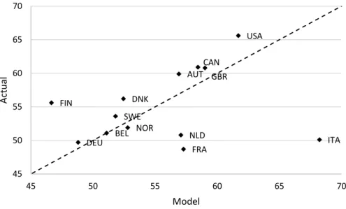
Figure 6.1 Employment rate in hours of young individuals (20-34), in %, 1995-2007.

Figure 6.2 Employment rate in hours of middle-aged individuals (35-49), in %, 1995- 2007.

Figure 6.3 Employment rate in hours of old individuals (50-65), in %, 1995-2007.

Figure 6.4 Tertiary education rate, in %, 1995-2007.

Figure 6.5 Annual per capita potential GDP growth, in %, 1995-2007.

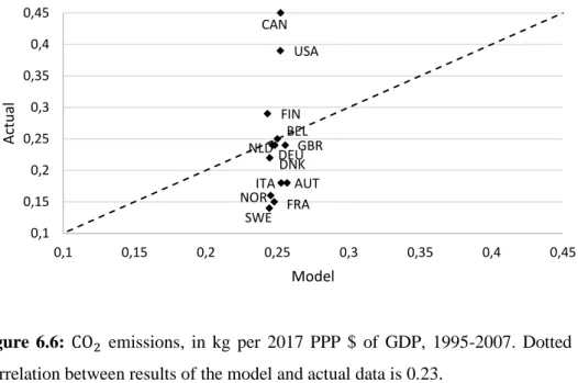
Figure 6.6 CO₂ emissions, in kg per 2017 PPP $ of GDP, 1995-2007.

Figure 8.1 Evolution of aggregate output level after a permanent environmental tax financed policy shock in period 1.

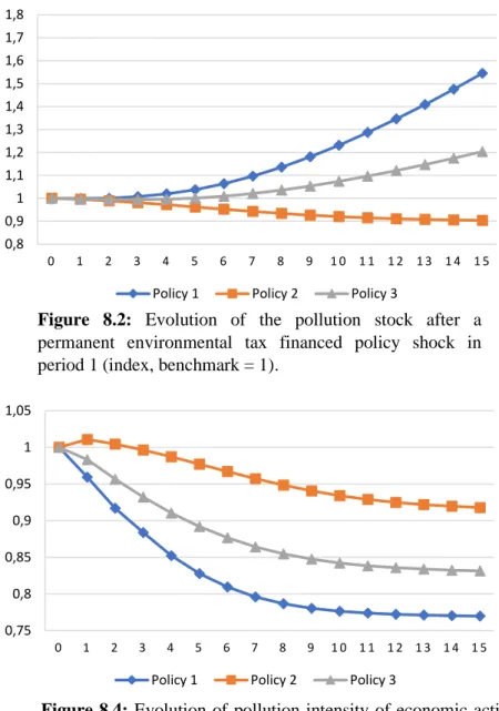
Figure 8.2 Evolution of the pollution stock after a permanent environmental tax financed policy shock in period 1.

Figure 8.3 Evolution of environmental capital after a permanent environmental tax financed policy shock in period 1.

Figure 8.4 Evolution of pollution intensity of economic activity (Pol/Y) after a permanent environmental tax financed policy shock in period 1.

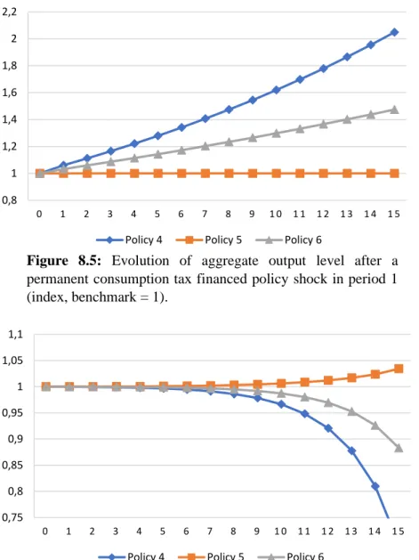
Figure 8.5 Evolution of aggregate output level after a permanent consumption tax financed policy shock in period 1.

Figure 8.6 Evolution of the pollution stock after a permanent consumption tax financed policy shock in period 1.

Figure 8.7 Evolution of environmental capital after a permanent consumption tax financed policy shock in period 1.

(8)

VII

Figure 8.8 Evolution of pollution intensity of economic activity (Pol/Y) after a permanent consumption tax financed policy shock in period 1.

Figure 8.9 Evolution of employment of young individuals after a temporary debt financed policy shock in period 1.

Figure 8.10 Evolution of employment of middle-aged individuals after a temporary debt financed policy shock in period 1.

Figure 8.11 Evolution of employment of older individuals after a temporary debt financed policy shock in period 1.

Figure 8.12 Evolution of aggregate employment after a temporary debt financed policy shock in period 1.

Figure 8.13 Evolution of the education rate after a temporary debt financed policy shock in period 1.

Figure 8.14 Evolution of the annual growth rate after a temporary debt financed policy shock in period 1.

Figure 8.15 Evolution of aggregate output level after a temporary debt financed policy shock in period 1.

Figure 8.16 Evolution of the pollution stock after a temporary debt financed policy shock in period 1.

Figure 8.17 Evolution of environmental capital after a temporary debt financed policy shock in period 1.

Figure 8.18 Evolution of pollution intensity of economic activity (Pol/Y) after a temporary debt financed policy shock in period 1.

Figure 9.1 Welfare implications for current and future generations of permanent higher government spending on climate mitigation and/or adaptation, financed by environmental taxes.

Figure 9.2 Welfare implications for current and future generations of permanent higher government spending on climate mitigation and/or adaptation, financed by consumption taxes.

(9)

VIII

Figure 9.3 Welfare implications for current and future generations of temporary higher government spending on climate mitigation and/or adaptation, financed by public debt.

Figure 10.1 Evolution of employment of young individuals after a temporary debt financed policy shock in period 1.

Figure 10.2 Evolution of employment of middle-aged individuals after a temporary debt financed policy shock in period 1.

Figure 10.3 Evolution of employment of older individuals after a temporary debt financed policy shock in period 1.

Figure 10.4 Evolution of aggregate employment after a temporary debt financed policy shock in period 1.

Figure 10.5 Evolution of the education rate after a temporary debt financed policy shock in period 1.

Figure 10.6 Evolution of the annual growth rate after a temporary debt financed policy shock in period 1.

Figure 10.7 Evolution of aggregate output level after a temporary debt financed policy shock in period 1.

Figure 10.8 Evolution of the pollution stock after a temporary debt financed policy shock in period 1.

Figure 10.9 Evolution of environmental capital after a temporary debt financed policy shock in period 1.

Figure 10.10 Evolution of pollution intensity of economic activity (Pol/Y) after a temporary debt financed policy shock in period 1.

Figure 10.11 Welfare implications for current and future generations of temporary higher government spending on climate mitigation and/or adaptation, financed by public debt.

(10)

IX

List of tables

Table 1 Overview of model parameters

Table 2 Policy parameters regarding government revenue

Table 3 Policy parameters regarding government spending and researchers

Table 4 Target values calibration

Table 5 Actual data for empirical test

Table 6 Overview policy scenarios

(11)

1

1. Introduction

On 11th December 2019 the European Commission presented the European Green Deal, a comprehensive plan to mitigate climate change in the following decades. The target for the European Union is to halve carbon emissions by 2030 and to become a carbon-neutral economy by 2050. Fiscal policy has an important role to play in this transition. There is an urgent need to better align taxation systems with climate objectives. These tax reforms will however not be sufficient. Major public investments in infrastructure, the energy sector and green technologies are needed as well. The Stern review, a landmark report on climate change, showed that the price of non-action is far greater than the cost of acting. If we do not act costs equivalent to at least 5% of global GDP each year will occur. These damages could rise to 20% of annual global GDP (Stern, 2007).

As the first concrete proposals for financing the European Green Deal investment plan were laid out by the European Commission, the COVID-19 outbreak struck the world economy. National governments reacted quickly by using fiscal instruments to soften the economic impact of the pandemic. A recent Oxford University paper on the climate impact of recovery packages warns that “there are reasons to fear that we will leap from the COVID frying pan into the climate fire” (Hepburn et al., 2020, p.4). In the coming weeks and months policymakers will shape recovery packages that could have a major impact on whether or not we will reach our climate targets. In the aftermath of the global financial crisis (hereafter “GFC”) stimulus packages were mainly ‘colourless’ meaning that they had no impact on greenhouse gas (hereafter “GHG”) emissions or even ‘brown’, which indicates that they were likely to increase GHG emissions (Hepburn et al., 2020). The current crisis is obviously different from the previous GFC, so other measures will be needed. Opting this time for predominantly green fiscal recovery packages can decouple future economic growth from GHG emissions.

The macroeconomic environment is characterised by a declining interest rate facing the effective lower bound. Due to structural causes - ageing societies, worldwide income- and wealth inequality, a global savings glut and a preference for safe assets by pension funds and insurance companies - interest rates are expected to remain low in the coming years

“A level-headed reassessment of public debt could lead to the green public investment necessary to fight climate change.” The Economist, July 25th 2020

(12)

2

(Jacobs, 2018). Advanced economies are in a state of secular stagnation and several economies could be dynamically inefficient (Summers, 2014; Geerolf, 2018). This means that fiscal and welfare cost of higher debt levels may be lower than assumed (Blanchard, 2019).

The current situation can be an opportunity for a debt financed increase in public spending in combination with a transition to a greener taxation system. In this master’s dissertation the impact of climate related government expenditures and its financing methods on key environmental, economic and welfare indicators are analysed within an overlapping generations (hereafter “OLG”) framework.

This master’s dissertation aims to answer two research questions. The first question this dissertation examines, is which public investments are essential for the climate transition? An important distinction to be made in this respect is the difference between climate change

mitigation measures to control and abate emissions, and climate change adaptation measures

to make the environment more resilient to global warming (IPCC, 2014). As climate mitigation measure we include productive government expenditures on green technology such as R&D investments and as adaptation measure public environmental capital investments for environmental resilience and regeneration. Both policy items are recommended by Hepburn et al. (2020) to be included in the coming fiscal recovery packages. The second question which is elaborated, is how should the government finance these extra climate related expenditures? Three different scenarios are taken into account: (1) a permanent environmental tax financed increase in government expenditures, (2) a permanent consumption tax financed increase in government spending, and (3) a temporary debt financed increase in public spending.

By using an OLG model that incorporates climate mitigation as well as adaptation spending and includes public debt in addition to tax revenue, this master’s dissertation tries to contribute to the existing literature on environmental fiscal policy. Next to a purely theoretical explanation of the model, we also perform specific policy simulations.

In the following section we first give an overview of existing literature on environmental issues in macroeconomic models. In section 3 the main causes of the current low interest rate and its consequences for public debt are explained. Section 4 describes the OLG model that will be used to analyse the different policies. The parameterisation of the model is explained in section 5. Before simulating several policy scenarios we perform an empirical test of the model to check its validity in section 6. In section 7 and 8 we analyse the results of policy simulations

(13)

3

by examining its numerical steady state effects and transitional dynamics of environmental and economic variables. Next to the analysis of these environmental and economic variables, we construct a welfare indicator to examine the welfare implications of policy changes in section 9. In section 10 the temporary debt financed policy changes are simulated for a lower interest rate environment, which characterises the current and future macroeconomic environment. Our conclusions are summarized in section 11.

(14)

4

2. Literature review

There is already a vast amount of macroeconomic literature on the impact of climate change. Nordhaus (1993) and Stern (2007) are two influential economists whose research gave shape to the economic climate policy debate in the last decade. They both use Integrated Assessment Models (hereafter “IAMs”) to measure the consequences caused by climate change and the cost of policy interventions to limit the damages. These models combine different strands in the literature to model economic decisions in combination with their impact on the environment, hence the reason why they are called “integrated” models. IAM is used to describe a wide range of macroeconomic models that can be different in complexity and working methods. Nordhaus (1993) works with a Dynamic Integrated model of Climate and the Economy (hereafter “DICE”), which is a simple IAM and approaches the economics of climate change from the perspective of neoclassical growth theory (e.g. Solow, 1970). According to these neoclassical growth models agents have to decide how much of their current income they consume and how much they invest in physical and human capital. The DICE model introduces natural capital as a third form of capital. GHG emissions have a negative impact on this natural capital. Agents can decide to reduce consumption today and invest in emission reduction, hereby preventing damages to natural capital and so increasing consumption in the future (Nordhaus & Sztorc, 2013).

Next to these structural macroeconomic models, there is a growing empirical literature that assesses the impact of climate change on growth. When deciding on which is the best policy to implement, it is crucial to incorporate empirical findings in the macroeconomic climate-economy models. Former president of the US, Barack Obama, stated in a policy note that models as the one used by Nordhaus (1993) “could substantially understate the potential damage of climate change on the global macroeconomy” (Obama, 2017, p.127). The source for this criticism is that those models do not account for the possibility of catastrophic events, such as thawing permafrost in Siberia that accelerates global warming or the increasing occurrence of extreme weather events such as cyclones and flooding (IPCC, 2012). Ecosystems often have critical tipping points. When such a tipping point is reached the state of the system may change drastically (Scheffer, 2009). Bakkensen and Barrage (2018) propose a new empirical-structural approach to close the “micro-macro” gap in the literature by integrating estimates for cyclone impacts on growth into the DICE model.

(15)

5

Climate change policy does not only focus on the impact on economic performance, but also has an important generational aspect. Policy changes can lead to financial transfers between generations; therefore OLG models as developed by Samuelson (1958), Diamond (1965) and Blanchard (1985) have an important function in the analysis and simulation of different policy proposals. In these models agents live a finite life and a clear distinction can be made between different generations as opposed to neoclassical growth models were agents live an infinite life and making distinctions between generations is not possible. This makes OLG models particularly suitable to assess the impact of environmental fiscal policies.

In these OLG models, the modelling of pollution can be separated in two main approaches. On the one hand, pollution can be the consequence of consuming (e.g. Habla & Roeder, 2013; John & Pecchenino, 1994). On the other hand, environmental deterioration can be caused by production. Bovenberg and Heijdra (1998) identify capital use as the source of pollution, while Palivos and Varvarigos (2010) mark pollution as an unfortunate by-product of production activities. Modelling pollution is not the only way to implement climate change in an OLG model. Several researchers introduce exhaustible natural resources in the production process (e.g. Howarth, 1991; Gerlagh & Keyzer, 2003). Another method is used by Catalano, Forni and Pezzolla (2020), with as basic assumption that climate change negatively influences the capital depreciation rate. This master’s dissertation uses an OLG model that incorporates several principles from earlier research. Both consumption and production are causes of pollution.

When we take a closer look at the possible fiscal policy instruments in environmental macroeconomic models, we can conclude that a large part of the literature exclusively focuses on taxation as fiscal policy instrument to influence climate change (e.g. Bovenberg & de Mooij, 1994; Goulder, 1995; Kirchner et al., 2019). One of the main findings is the possibility of a double dividend which was mentioned for the first time by Tullock (1967). He argued that taxing undesirable activities - he uses the example of congestion on highways – might offer two benefits. The cost of the tax is offset by the gain of less congestion (the first dividend). The tax revenue can be seen as a free good to the state (the second dividend). In the case of climate policy the double dividend hypothesis can be explained as follows: environmental taxes can reduce pollution which leads to an increase in environmental quality for future generations (first dividend), the revenues of a non-distortionary tax can be used to lower or displace other more distortionary taxes such as an income tax (second dividend). This is called the revenue recycling effect which results in a lower excess burden of taxation on the economy and enhances employment and economic growth.

(16)

6

Public debt is an important part of fiscal policy, and together with environmental taxes it can be used in the implementation of environmental fiscal reform. Heijdra, Kooiman and Ligthart (2006) introduce environmental externalities in a Yaari-Blanchard model - an OLG model in which agents have an uncertain lifetime - for a small open economy to study intergenerational effects of an increasing environmental tax, in this case a tax on capital income. Old existing generations are affected the most by the environmental tax, because they see a fall in their capital income. Karp and Rezai (2014) use another approach. They introduce an environmental ad valorem tax on the production of resource-intensive goods in their two-sector OLG model. Here the young generation bears the tax-induced costs and the welfare of the old and future generation increases. Although Heijdra et al. (2006) find different generational welfare implications, both studies argue that redistributive measures such as an accompanying public debt policy or intergenerational transfers can improve the welfare of all generations. Such pareto-improvements should lead to a wide support for environmental fiscal reforms.

As mentioned in the introduction, government policies regarding climate change are either considered climate mitigation measures to prevent and reduce GHG emissions or climate adaptation measures to adjust our economy and become more resilient towards global warming. Most environmental macroeconomic models only consider mitigation measures as policy option. However, adaptation measures have become part of the policy mix in more recent macroeconomic models. Bosello (2010) extends the DICE framework of Nordhaus and Sztorck (2013) to prove that mitigation and adaptation are both vital within environmental policy. Catalano et al. (2020) evaluate the role of fiscal policy in climate change adaptation within an OLG model. They conclude that a comprehensive strategy containing preventive (mitigation) as well as corrective (adaptation) measures is the most desirable outcome. In the OLG model used in this master’s dissertation a rich policy mix of taxation and government spending is included. Both mitigation and adaptation spending play their role.

To conclude this section, it is important to mention that there is considerable criticism on the “orthodox” macroeconomic models and the way these models integrate climate change. Neoclassical assumptions such as the homo economicus hypothesis, the handling of environmental damage as an externality that needs to be internalized and the unlimited growth possibility are subject of debate among economists today. Ecological macroeconomics is a new field that arose out of these debates. It combines elements of post-Keynesian economics (e.g. Kaldor, 1957) and ecological economics (e.g. Daly, 1968; Constanza et al., 1997). A promising new model in this line of research is the EUROGREEN model from D’Alessandro

(17)

7

et al. (2020), which involves a complex structure of system dynamics1 and a rich set of policy tools to simulate different strategies.

This increasing diversity in environmental macroeconomic models is beneficial for future research. A more interdisciplinary approach which contains different perspectives to tackle environmental issues is enriching the policy debate. The multifaceted approach stands at the core of ecological economics, encapsulated in Blanchard’s comment that “No model can be all things to all people” (Blanchard, 2018, p. 43).

1_{System dynamics: modelling strategy to evaluate the interconnections and feedback loops between}

(18)

8

3. Public debt in low interest rate environment

Before we explain our OLG model in the next section, we discuss the role public debt can play in fiscal policies, and more specifically the current debate around public debt in a low interest rate environment. As shown in Figure 1, nominal long-term interest rates on government bonds have been declining for decades. It could be the perfect moment to boost the transition towards a carbon-neutral economy with expansionary fiscal policy. International institutions as the IMF indicate that increased public infrastructure investment are needed (IMF, 2014). First, we will explain the dynamics of public debt based on Baert et al. (2020), Bouabdallah et al. (2017) and Heylen, Hoebeeck and Buyse (2011). Secondly, we specify the reasons for the downward trend in the interest rate. The last subsection gives an overview of the arguments made by the proponents of debt financed public investments, followed by some counterarguments.

3.1 Debt dynamics

The dynamics of a country’s debt-to-GDP ratio is given in Equation (a)2 and depends on the following variables: the primary balance in % of GDP (𝑝𝑏_𝑡), the nominal interest rate on outstanding debt in year t (𝑟_𝑛,𝑡), growth rate of nominal GDP in year t (𝑔_𝑛,𝑡), the ratio of nominal public debt in t-1 (𝑏_𝑡−1) and the stock-flow adjustment in year t in % of GDP (𝑠𝑓_𝑡).

Figure 1: Nominal long-term interest rates on government bonds maturing in ten years.

Source: OECD, General Statistics.

2_{The derivation of this equation is provided in Appendix 2.}

0 2 4 6 8 10 12 14 16

(19)

9

The primary balance is the difference between the government revenues and government expenditures, excluding interest rate payments. The stock-flow adjustment is a residual term that captures the effect on the debt-to-GDP ratio from accumulation of financial assets and the remaining statistical adjustments.

∆𝑏_𝑡 = −𝑝𝑏_𝑡+ (𝑟𝑛,𝑡− 𝑔𝑛,𝑡)

(1+ 𝑔𝑛,𝑡) 𝑏𝑡−1+ 𝑠𝑓𝑡 (a)

𝑏∗ = _𝑔𝑛−𝑝𝑏_{∗ −𝑟𝑛∗}∗

1+ 𝑔𝑛∗

(b)

With: “*” indicating long-term values

In our analysis of the dynamics of public debt we assume that the stock-flow adjustment term is zero. In a scenario where the nominal interest rate is larger than the nominal growth rate, a primary surplus (positive primary balance) is needed to stabilize the debt-to-GDP ratio. A primary deficit in this macroeconomic situation would result in a snowball effect that leads to a continuous increase in the debt-to-GDP ratio.

When the nominal interest rate is lower than the nominal growth rate, there can be a stable debt ratio whilst having a primary deficit. Starting from Equation (a) we can determine the stable long-term debt ratio (Equation b), whereby temporary higher government investment leading to high primary deficits will not result in a higher debt-to-GDP ratio in the long-run. The reason being that GDP (denominator of the ratio) grows faster than the total amount of debt (numerator of the ratio).

The current macroeconomic environment can be described by the second scenario. The interest rate on government bonds is lower than the long-term nominal growth rate in all major advanced economies (Blanchard, 2019).

3.2 Drivers of the low interest rate

There are several structural causes for the decline of the long-term interest rate on government bonds. Summers (2015) argues that structurally high private savings and low demand for investments put downward pressure on the interest rate and can bring economies in a situation of secular stagnation (long period of low economic growth and very low interest rates)3.

(20)

10

One cause of this increase in private savings are demographic developments. Due to a longer life expectancy, individuals will save more. They anticipate a longer retirement period (Carvalho, Ferrero & Nechio, 2016). A decline in the population growth also has a negative effect on the marginal product of capital, leading to less investments. Another cause is the rise in income and wealth inequality. The income distribution has become more unequal in most advanced economies over the last decades. High wage earners have a higher propensity to save (Carvalho & Rezai, 2016). Thus, growing inequality results in lower aggregate demand and higher savings. High income inequality and changing demographics are two factors that will not disappear in the near future. The downwards pressure they put on nominal interest rates will persist in the time to come.

The growing demand for safe assets, such as government bonds, leads to a further decline of the interest rate on public debt (Caballero, Farhi & Gourinchas, 2017). Safe assets are becoming scarce, which means investors will accept a lower interest rate.

3.3 Time for fiscal expansion

A drop in consumption and increased savings result in a lower rate of return on capital, which will encourage individuals to save even more. This effect is known as the paradox of thrift and could make an economy dynamically inefficient. A reduction in the savings rate would improve the welfare of future and current generations. Rachel and Summers (2019) argue that higher deficits and structural policies to promote investment and/or reduce private savings are needed to escape a situation where output is demand constrained.

When economies are confronted with a binding zero lower bound4 (hereafter “ZLB”) on interest rates, Say’s law – supply always creates its own demand – no longer holds (Jacobs, 2020). In a ZLB environment the fiscal and welfare cost of higher public debt could be lower than expected (Blanchard, 2019). The Japanese economy has been confronted with the ZLB since the mid-1990’s. Evidence for Japan suggests that the output multiplier of government spending is larger during periods where the economy is confronted with the ZLB (Miyamoto, Nguyen & Sergeyev, 2018).

4_{The zero lower bound refers to a situation where the short-term nominal interest rates are at or near zero. There}

is debate among economists about the effectiveness of monetary policies around or below the ZLB. For a discussion on monetary policy at the ZLB, see Bernanke and Reinhart (2004).

(21)

11

Ubide (2016) identifies different ways in which an expansionary fiscal stance can create positive effects on economic performance. The first effect is a productivity increase caused by public investments that boost potential growth. An increase in government investments yields positive demand effects and increases the stock of public capital, which contributes to the economy’s output potential (ECB, 2016). DeLong and Summers (2012) state that government investments which support potential growth can be self-financing. The IMF argues that “debt financed projects could have large output effects without increasing the debt-to-GDP ratio, if clearly identified infrastructural needs are met through efficient investments” (IMF, 2014, p. 75). These infrastructural investments are an opportunity to make our infrastructure more energy efficient. However, since the late 1970’s the public capital stock is declining in most OECD countries (Kamps, 2006). In Belgium, general government investments have decreased from 5% of GDP in 1970 to 2,4% in 2015 (Biatour et al., 2017). Another positive effect of expansionary fiscal policy according to Ubide (2016) is its ability to increase the effectiveness of monetary policy. Fiscal expansion increases the supply of government bonds and reduces the scarcity of safe assets.

Contrasting with these arguments in favour of fiscal expansion, Blanchard (2019) lists three counterarguments that may increase the potential costs of public debt. (1) Due to financial distortions such as the obligation for financial institutions to hold a particular proportion of government bonds in their portfolios, the rate on government bonds may be artificially low. If this is the case, diminishing the financial distortions and so giving financial institutions the possibility to increase corporate lending would augment private capital formation (Becker & Ivashina, 2018) and be welfare increasing in general. However, a side effect of the elimination of these obligations could be an increase in the public debt servicing costs. (2) The future is uncertain. Some factors that have a downward effect on the interest rate may disappear over time, or the increase in public debt leads to a crowding out of private capital and subsequently to a higher marginal product of capital up to the point where the interest rate on public debt exceeds the growth rate. (3) Higher public debt can lead to multiple fiscal equilibria. Investors could regard public debt to be a safe asset and accept a lower interest rate, or government debt could be perceived as risky. In the latter case investors will demand a risk premium, which enhances the costs of public debt.

Taking the whole range of possible advantages, opportunities and risks into account, Blanchard and Ubide (2019) conclude that fiscal policy should tilt in a more expansionary direction.

(22)

12

4. The benchmark model

This section explains the basic set-up of the analytical model that will be used for policy analysis. First household preferences, human capital formation and the optimisation problem of individuals are explained. Secondly, the production functions of intermediate and final good producers and their demand for labour and capital are described. The next subsection illustrates how the environment enters the model, followed by a subsection on the government sector. A final subsection focuses on aggregate equilibrium.

4.1 Introduction: basic set-up and characteristics of the model

Our analytical framework borrows heavily from Rabaey (2019) and Heylen and Van de Kerckhove (2013). The benchmark model is a four-period overlapping generations model for an open economy. Perfect international mobility of physical capital but immobile labour and human capital is assumed. The model consists of four generations, which are divided in two categories. The first category is the active population (20-64 year) and contains three generations: the young (age 20-34), middle-aged (age 35-49) and older (age 50-64) workers. The second category contains one generation of retired individuals (65-79 year). Agents enter the model at the age of 20, each subsequent period consists of 15 years. Young individuals divide their time between work, leisure and education. The middle-aged and older individuals in the active population divide their time between work and leisure. Agents retire at the age of 65; an early retirement is no option in this framework. All generations are of equal size and normalised to 1. This means that there is no population growth in the model; total population is 4 and remains constant. The domestic final good producers operate on a perfectly competitive market. They use clean (pollution free) and dirty (pollution intensive) inputs that are made by intermediate good producers on an imperfectly competitive market. The intermediate good producers employ physical capital together with existing technology and human capital provided by the three active generations. The government receives revenues from consumption, capital, labour and environmental taxes. A balanced budget is not imposed, the government can borrow and accumulate debt.

The variables in the equations of this section use several super- and subscripts. Superscript t refers to the period in which the agent is introduced in the model, t stands for the particular generation of this agent. Subscript j on the other hand indicates the age group in which the individual is situated, at working age (young, middle-aged, older) or retired. In general

(23)

13

aggregate variables, such as wages, interest rates and output, have time subscripts which demonstrate historical time.5

4.2 Households

4.2.1 Preferences and time allocation

An individual reaching the age of 20 in period t maximises a lifetime utility function of the form: 𝑈𝑡 _{= ∑} _𝛽𝑗−1_{(𝑙𝑛 𝑐} 𝑗𝑡+ 𝛾𝑗 1−𝜃 4 𝑗=1 (𝑙𝑗𝑡)1−𝜃+ 𝜈 𝑙𝑛 𝐸𝑡+𝑗−1) . (1) With 0 < β < 1, 𝛾𝑗 > 0, 𝜈 > 0, and θ > 0 (θ ≠ 1)

The households create utility out of consumption (𝑐_𝑗𝑡), leisure (𝑙_𝑗𝑡) and an environmental capital stock variable (𝐸𝑡+𝑗−1), which is a proxy for the quality of the environment around the

households and its resilience to climate change, during the four periods in the model. The discount factor (𝛽𝑗−1_{) brings future consumption, leisure and environmental conditions to the}

present. We use preference parameters, 𝛾_𝑗 for leisure and 𝜈 for the environment, to be able to reveal relative preference between the three components of lifetime utility. 𝛾_𝑗 is allowed to vary by age group, while 𝜈 is kept constant over the individual’s lifetime. The intertemporal elasticity of substitution in leisure is 1/𝜃. A high 𝜃 results in a low elasticity of substitution in leisure, a low 𝜃 in a high one. The larger the elasticity of substitution the more easily an individual changes its leisure over time. The intertemporal elasticities in consumption and the environment are both one, due to the logarithmic specification.

Equations (2) – (5) show how the representative individual of generation t divides his or her time in each of the four periods of life. The total amount of time to spend in each period is normalised to 1.

𝑙₁𝑡 = 1 − 𝑛₁𝑡 − 𝑒₁𝑡 (2)

𝑙₂𝑡 = 1 − 𝑛₂𝑡 (3)

5_{Two examples:}

1) 𝑒1𝑡 indicates the time an individual, who enters the model at time t (superscript t), spends on education when

this individual is young (subscript 1). This will happen in historical period t. 2) 𝑌_𝑡+2 is the macroeconomic output in period t+2 (historical time, subscript t+2)

(24)

14 𝑙₃𝑡 _{= 1 − 𝑛}

3𝑡 (4)

𝑙₄𝑡 _{= 1} ₍₅₎

Figure 2 gives an overview of the time allocation over the life cycle of an individual of generation t. When young the individual has to divide his or her time between work, leisure and education. In the second and third period education is no longer an option, hence the individual divides his or her time between work and leisure. In the last period, after retiring at 65, the individual devotes all of his or her time to leisure.

20 35 50 65 80

Period t t + 1 t + 2 t + 3

Work 𝑛1𝑡 𝑛2𝑡 𝑛3𝑡 0

Study 𝑒1𝑡 0 0 0

Leisure 1 − 𝑛₁𝑡− 𝑒₁𝑡 1 − 𝑛₂𝑡 1 − 𝑛₃𝑡 1

Figure 2: Time allocation over the life cycle of an individual of generation t.

4.2.2 Budget constraints

Equations (6) – (9) represent the budget constraints that the representative individual of generation t encounters in each period of his or her life.

(1 + 𝜏_𝑐) 𝑐₁𝑡_{+ 𝑎} 1𝑡 = 𝑤𝑡ℎ1𝑡𝑛1𝑡(1 − 𝜏𝑤) + 𝑏𝑤𝑡ℎ1𝑡(1 − 𝑛1𝑡− 𝑒1𝑡)(1 − 𝜏𝑤) + 𝑑𝑡+ 𝑧𝑡 (6) (1 + 𝜏𝑐) 𝑐2𝑡+ 𝑎2𝑡 = 𝑤𝑡+1ℎ2𝑡𝑛2𝑡(1 − 𝜏𝑤) + 𝑏𝑤𝑡+1ℎ2𝑡(1 − 𝑛2𝑡)(1 − 𝜏𝑤) + 𝑑𝑡+1+ 𝑧𝑡+1 (7) + (1 + 𝑟𝑡+1(1 − 𝜏𝑘))𝑎1 𝑡 𝑃𝑡 𝑃𝑡+1 (1 + 𝜏𝑐) 𝑐3𝑡+ 𝑎3𝑡 = 𝑤𝑡+2ℎ3𝑡𝑛3𝑡(1 − 𝜏𝑤) + 𝑏𝑤𝑡+2ℎ3𝑡(1 − 𝑛3𝑡)(1 − 𝜏𝑤) + 𝑑𝑡+2+ 𝑧𝑡+2 (8) + (1 + 𝑟_𝑡+2(1 − 𝜏_𝑘))𝑎₂𝑡 𝑃𝑡+1 𝑃𝑡+2 (1 + 𝜏𝑐) 𝑐4𝑡= 𝑝𝑝4𝑡+ 𝑑𝑡+3+ 𝑧𝑡+3+ (1 + 𝑟𝑡+3(1 − 𝜏𝑘))𝑎3 𝑡 𝑃_𝑃𝑡+2 𝑡+3 (9)

The right hand side (hereafter “RHS”) of Equations (6) – (9) identifies the disposable resources the individual has in each period. A first component is his or her real after-tax labour income,

(25)

15

it depends on the real wage rate per unit of effective labour (𝑤_𝑡), effective human capital (ℎ_𝑗𝑡) and hours worked (𝑛_𝑗𝑡). Another component are non-employment benefits, which are a fraction (𝑏) of real after-tax labour income. The active generations receive these benefits for the fraction of time that they are inactive. In the last period, when the individual is retired, these first two components are replaced by a public pension (𝑝𝑝₄𝑡_{). A third and fourth component are dividends}

that the individual receives from ownership of the firms (𝑑_𝑡) and a lump sum transfer (𝑧_𝑡) from the government. A last component is the real interest income on accumulated savings (𝑎_𝑗𝑡) after subtracting the capital tax (𝜏𝑘) levied by the government. Changes in the price level (𝑃𝑡)

influence the real value of interest income on assets accumulated in the previous period. The left hand side (hereafter “LHS”) of Equations (6) – (9) demonstrates where the individual’s resources go to. When the individual is at working age, disposable resources are divided between consumption (𝑐_𝑗𝑡), including the consumption tax (𝜏_𝑐), and accumulated assets or non-human wealth (𝑎_𝑗𝑡). Accumulated assets are measured at the end of each period. In the last period the individual consumes all of his or her resources, no savings or debts are left for future generations.

Equation (10) defines the public pension that individuals receive when they retire. The size of the public pension is a fraction (𝑏4) of the average after-tax labour income in the three previous

periods. The pension rises in hours worked, human capital and the real wage in earlier periods. A higher labour tax leads to a lower pension. The public pensions are financed through a PAYG (pay as you go) system. The labour tax contributions of the active generations serve as resources for the public pensions. Most OECD countries have a PAYG type pension system.

𝑝𝑝₄𝑡 _{= 𝑏} 4∑ 1 3 3 𝑗=1 (𝑤𝑡+𝑗−1ℎ𝑗𝑡𝑛𝑗𝑡(1 − 𝜏𝑤)) (10)

4.2.3 Human capital formation

Equation (11) - (12) demonstrate the evolution of human capital over the life cycle of an individual of generation t. The model has a simple human capital function similar to the one in Lucas (1990) and Buyse, Heylen and Van de Kerkchove (2017). The representative individual enters the model at the age of 20 with a predetermined level of human capital (ℎ₁𝑡), which is generation-invariant. We normalise the level of human capital in the first period to 1. When young, the individual can invest in education and increase his or her level of human capital. The new level is determined by the previous level of human capital, the time the individual

(26)

16

spends on education during the first period (𝑒₁𝑡_{), the elasticity of time input (𝜎) and a positive}

efficiency parameter (𝜑). Equation (12) shows that there is no depreciation of human capital between the second and third period; the level remaining unchanged.

ℎ₁𝑡 = 1 (11)

ℎ₂𝑡 = ℎ₃𝑡 = ℎ₁𝑡(1 + 𝜑(𝑒₁𝑡₎𝜎₎ ₍₁₂₎

With 0 < 𝜎 ≤ 1, 𝜑 > 0

4.2.4 Optimisation

An individual chooses his or her consumption, leisure and time on education in order to maximise lifetime utility. We substitute Equations (2) – (4) for leisure and the budget constraints (6) – (9) for consumption into Equation (1). After constructing a Lagrangian and maximising with respect to 𝑎₁𝑡, 𝑎₂𝑡, 𝑎₃𝑡, 𝑛₁𝑡, 𝑛₂𝑡, 𝑛₃𝑡 and 𝑒₁𝑡, we obtain seven first-order conditions for the optimal behaviour of an individual of generation t. From these first-order conditions optimal consumption, optimal labour supply and the optimal time on education can be derived.

Equation (13) describes the law of motion of optimal consumption over time. Consumption in the next period will be higher than current consumption if the after-tax interest rate (1 + 𝑟_𝑡+𝑗(1 − 𝜏𝑘)) is higher than the inverse of the discount factor (𝛽)6.

𝑐_𝑗+1𝑡 𝑐_𝑗𝑡

𝑃_𝑡+𝑗𝑡

𝑃_{𝑡+𝑗−1}𝑡 = 𝛽 (1 + 𝑟𝑡+𝑗(1 − 𝜏𝑘)) ∀ 𝑗 = 1, 2, 3 (13)

Equations (14) – (16) express the optimal labour supply in each of the three active periods in an individual’s life. In each period, individuals offer their labour up to the point where the marginal utility of leisure equals the marginal utility of work. The LHS represents the utility loss from working an extra hour. Working more leads to less leisure and by consequence less utility. The RHS shows the marginal utility gain from working an extra hour. Supplying more hours of labour leads to a higher income and public pension, which results in more consumption in the current period and when the individual is retired. Individuals have a stronger incentive to work when the initial consumption is lower and when working an extra hour results in a stronger

6_{𝛽 =} 1

(27)

17

rise in consumption. This situation occurs if human capital (ℎ₁𝑡_{), the real wage (𝑤}

𝑡+𝑗−1) and

the pension replacement rate (𝑏₄) are high. A stronger increase in consumption will also appear when consumption taxes (𝜏_𝑐), non-employment benefits (𝑏) and/or taxes on labour (𝜏_𝑤) are low. 𝛾1 (𝑙1𝑡)𝜃 −𝜕𝑙1𝑡 𝜕𝑛1𝑡 = 𝑤𝑡ℎ1𝑡(1− 𝜏𝑤)(1−𝑏) 𝑐1𝑡(1+ 𝜏𝑐) + 𝛽3 3 𝑏4𝑤𝑡ℎ1𝑡(1− 𝜏𝑤) 𝑐4𝑡(1+ 𝜏𝑐) (14) 𝛾2 (𝑙₂𝑡)𝜃 −𝜕𝑙2𝑡 𝜕𝑛₂𝑡 = 𝑤𝑡+1(1 + 𝜑(𝑒1𝑡) 𝜎 )ℎ1𝑡(1− 𝜏𝑤)(1−𝑏) 𝑐₂𝑡(1+ 𝜏𝑐) + 𝛽2 3 𝑏4𝑤𝑡+1(1 + 𝜑(𝑒1𝑡) 𝜎 )ℎ1𝑡(1− 𝜏𝑤) 𝑐₄𝑡(1+ 𝜏𝑐) (15) 𝛾3 (𝑙₃𝑡)𝜃 −𝜕𝑙3𝑡 𝜕𝑛₃𝑡 = 𝑤𝑡+2(1 + 𝜑(𝑒1𝑡) 𝜎 )ℎ1𝑡(1− 𝜏𝑤)(1−𝑏) 𝑐₃𝑡(1+ 𝜏𝑐) + 𝛽 3 𝑏4𝑤𝑡+2(1 + 𝜑(𝑒1𝑡) 𝜎 )ℎ1𝑡(1− 𝜏𝑤) 𝑐₄𝑡(1+ 𝜏𝑐) (16)

Equation (17) describes the optimal level of education. The LHS is the marginal utility loss from investing an extra hour in education when young. An extra hour of study leads to less leisure or less labour, which results in less consumption. The RHS is the discounted marginal utility gain from higher human capital in the following two active periods and in retirement. Extra human capital increases labour income in the second and third period, and also increases the public pension. Higher labour taxes in the first period decrease the cost of studying an extra hour, which will encourage individuals to allocate more time to education. Higher taxes on labour income in later periods of life, however, will do the opposite. They reduce the return to accumulated human capital. Interesting to mention is that young people will also study more if they expect to spend a higher portion of their time working in later periods.

𝛾1 (𝑙₁𝑡)𝜃 −𝜕𝑙1𝑡 𝜕𝑒₁𝑡 − 1 𝑐₁𝑡 𝜕𝑐1𝑡 𝜕𝑒₁𝑡 = 𝛽 1 𝑐₂𝑡 𝜕𝑐2𝑡 𝜕𝑒₁𝑡 + 𝛽 2 1 𝑐₃𝑡 𝜕𝑐3𝑡 𝜕𝑒₁𝑡 + 𝛽 3 1 𝑐₄𝑡 𝜕𝑐4𝑡 𝜕𝑒₁𝑡 (17) With: 𝜕𝑐1𝑡 𝜕𝑒1𝑡= −𝑏𝑤𝑡ℎ1𝑡(1− 𝜏𝑤) 1+ 𝜏𝑐 𝜕𝑐2𝑡 𝜕𝑒₁𝑡= 𝜎𝜑(𝑒1 𝑡₎𝜎−1_.𝑤𝑡+1ℎ1𝑡(1− 𝜏𝑤)(𝑛2𝑡+ 𝑏(1− 𝑛2𝑡)) 1+ 𝜏𝑐 𝜕𝑐3𝑡 𝜕𝑒1𝑡= 𝜎𝜑(𝑒1 𝑡₎𝜎−1_.𝑤𝑡+2ℎ1𝑡(1− 𝜏𝑤)(𝑛3𝑡+ 𝑏(1− 𝑛3𝑡)) 1+ 𝜏𝑐 𝜕𝑐4𝑡 𝜕𝑒1𝑡= 𝑏4 3 . 𝜎𝜑(𝑒1 𝑡₎𝜎−1_.∑ (𝑛𝑗 𝑡_𝑤 𝑡+𝑗−1ℎ1𝑡(1− 𝜏𝑤)) 3 𝑗=2 1+ 𝜏𝑐

(28)

18 4.3 Firms, output and factor prices

4.3.1 Production of final goods

Domestic final good producers operate on a perfectly competitive market and produce the final good (𝑌_𝑡) according to a constant elasticity of substitution (CES) production function as in Equation (18). Final good producers use two kinds of intermediate goods in their production. One clean7 input (𝑋_𝐶𝑡) that does not produce damaging emissions in the production process and one dirty input (𝑋𝐷𝑡) that causes harmful pollution. Firms can change their production process

and switch dirty inputs for clean ones, but this comes with a price. The interchangeability between the two intermediate goods is given by the elasticity of substitution (𝜀). 𝜂 is a share parameter. 𝑌_𝑡 = (𝜂𝑋_𝐶𝑡 𝜀−1 𝜀 _{+ (1 − 𝜂)𝑋} 𝐷𝑡 𝜀−1 𝜀 ₎ 𝜀 𝜀−1 (18)

Final goods producers will maximise their profits according to Equation (19). 𝑃_𝑡 is the aggregate price level, 𝑃_𝐶𝑡 the price for a clean intermediate good and 𝑃_𝐷𝑡 the price for a dirty intermediate input. Prices of the intermediate goods are determined by the intermediate goods producers. The government levies an environmental tax (𝜏𝐷) on the dirty intermediate good

(𝑋_𝐷𝑡). Solving the maximisation problem results in a demand for the intermediate goods given by Equations (20) - (21)8. The intermediate good producers adjust their production to meet the demand for both intermediate inputs.

max 𝑋𝐶𝑡,𝑋𝐷𝑡 𝑃_𝑡𝑌_𝑡− 𝑃_𝐶𝑡𝑋_𝐶𝑡 − (1 + 𝜏_𝐷)𝑃_𝐷𝑡𝑋_𝐷𝑡 (19) 𝑋𝐶𝑡 = ( 1 𝜂) −𝜀 (𝑃𝐶𝑡 𝑃𝑡) −𝜀 𝑌𝑡 (20) 𝑋_𝐷𝑡 = ( 1 1− 𝜂) −𝜀 ((1+ 𝜏𝐷)𝑃𝐷𝑡 𝑃𝑡 ) −𝜀 𝑌_𝑡 (21)

7_{The property clean given to production inputs in this and following sections means pollution-free. The}

adjective dirty implies pollution-intensive inputs.

(29)

19

4.3.2 Production of intermediate goods

Domestic intermediate good producers operate on a imperfectly competitive market and produce the intermediate goods (𝑌_𝐶𝑡, 𝑌_𝐷𝑡) according to Cobb-Douglas production functions as in Equations (22) - (23). 𝐵_𝐶𝑡 and 𝐵_𝐷 are sector-specific technology parameters. Technology used for the production of dirty intermediate goods is time-invariant. The technology parameter in the production of the clean intermediate good changes over time (see Equation 24). 𝐾𝐶𝑡 and

𝐾_𝐷𝑡 are the sector-specific physical capital stocks. 𝐻_𝐶𝑡 and 𝐻_𝐷𝑡 represent sector-specific effective labour.

𝑌_𝐶𝑡 = 𝑋_𝐶𝑡 = 𝐾_𝐶𝑡𝛼_(𝐵

𝐶𝑡𝐻𝐶𝑡)1−𝛼 (22)

𝑌_𝐷𝑡 = 𝑋_𝐷𝑡 = 𝐾_𝐷𝑡𝛼(𝐵𝐷𝐻𝐷𝑡)1−𝛼 (23)

Equation (24) describes the change in 𝐵_𝐶𝑡 over time. Productive government expenditures (𝐺𝑦1𝑡) improve clean technologies (R&D on green production technologies and investments in

technologies that generate sustainable energy such as solar panels, hydropower plants and windmills). 𝑔𝑦1 is defined as a fixed fraction of output (𝑌𝑡) that the government spends on the

improvement of green technology. These productive government expenditures are marked as climate mitigation investments, used to control and abate pollution9. A second variable that influences the level of clean technology is the ratio of researchers per thousand employed individuals (𝑟𝑠). The effectiveness of productive government expenditures and researchers in the improvement of clean technologies is determined by 𝜔. 𝜅 and (1 − 𝜅) are the elasticities of respectively productive government spending and researchers with respect to green technology. 𝐵_𝐶𝑡 = 𝐵_𝐶𝑡−1(1 + 𝜔(𝑔_𝑦1)𝜅_(𝑟𝑠)1−𝜅₎ ₍₂₄₎ With: 0 < 𝜅 < 1, 𝑔_𝑦1 = 𝐺𝑦1𝑡 𝑌𝑡 9_{We refer to 𝐺}

𝑦1𝑡 in this master’s dissertation as productive government expenditures on green/clean technology

(30)

20

Clean (C) and dirty (D) intermediate good producers will demand an amount of effective labour and physical capital that minimises their production costs. After constructing a Lagrangian (Equation 25) and solving the first-order conditions, Equation (26) – (27)10 give respectively the optimal demand for effective labour and physical capital in both intermediate good sectors.

ℒ = 𝑤_𝑡𝐻_𝑠𝑡+ (𝑟_𝑡 + 𝛿_𝑘) 𝐾_𝑠𝑡+ 𝜆_𝑡(𝑌_𝑠𝑡− 𝐾_𝑠𝑡𝛼(𝐵_𝑠𝑡𝐻_𝑠𝑡)1−𝛼_{) ∀ 𝑠 = 𝐶, 𝐷} ₍₂₅₎ 𝐻𝑠𝑡 = 𝑌𝑠𝑡 𝐵𝑠𝑡1−𝛼 ( 1− 𝛼 𝛼 ) 𝛼 ( 𝑤𝑡 𝑟𝑡+ 𝛿𝑘) −𝛼 ∀ 𝑠 = 𝐶, 𝐷 (26) 𝐾_𝑠𝑡 = 𝑌𝑠𝑡 𝐵𝑠𝑡1−𝛼 (1− 𝛼 𝛼 ) (𝛼−1) ( 𝑤𝑡 𝑟𝑡+ 𝛿𝑘) (1−𝛼) ∀ 𝑠 = 𝐶, 𝐷 (27)

The common wage in both intermediate good sectors is determined through the equality of total effective labour demand (Equation 28) and effective labour supply (Equation 29). Total effective labour demand is the sum of optimal effective labour demand in the clean and dirty intermediate good sector. Effective labour supply is the total amount of time that all individuals in the active population work at time t. Individuals choose their labour supply optimally following Equations (14) – (16) (supra).

𝐻_𝐶𝑡 + 𝐻_𝐷𝑡 = ( 𝑌𝐶𝑡 𝐵_𝐶𝑡1−𝛼 + 𝑌𝐷𝑡 𝐵_𝐷1−𝛼) (( 1− 𝛼 𝛼 ) 𝛼 ( 𝑤𝑡 𝑟𝑡+ 𝛿𝑘) −𝛼 ) (28) 𝐻𝑡 = 𝑛1𝑡ℎ1𝑡+ 𝑛2𝑡−1ℎ2𝑡−1+ 𝑛3𝑡−2ℎ3𝑡−2 (29)

The intermediate good firms operate in a small open economy, by consequence the firms have no influence on the real interest rate. The world real interest rate (𝑟_𝑡) is exogenously determined. A lower depreciation rate of physical capital or higher wages, given the real interest rate, will lead to a higher demand for physical capital by the intermediate good firms. The first graph in Figure 3 illustrates the formation of the real wage and the aggregate level of effective labour that the intermediate good firms use. A higher wage leads to a higher aggregate supply of labour, but the optimal demand for labour in each sector decreases. The labour supply curve shifts to the right if the current active generations work more hours (𝑛₁𝑡, 𝑛₂𝑡−1, 𝑛₃𝑡−2) or their human capital (ℎ₁𝑡, ℎ₂𝑡−1, ℎ₃𝑡−2) increases. The labour demand curve moves to the right if the production of intermediate goods (𝑌𝑠𝑡) goes up or when the cost of capital (𝑟𝑡+ 𝛿𝑘) rises.

(31)

21

Figure 3: Determination of employment, the real wage and installed physical capital.

Labour demand shifts to the left if the level of technology in the intermediate good production functions (𝐵_𝑠𝑡) increases. The equality of supply and demand for labour results in a unique real wage. The second graph in Figure 3 shows how the amount of physical capital, used by the intermediate good firms, is determined. The world interest rate is given exogenously and might change over time. The demand for physical capital shifts to the right if the production of intermediate goods (𝑌_𝑠𝑡) rises or when the real wage (𝑤_𝑡) increases. Physical capital demand moves to the left if the level of technology in the intermediate good production functions (𝐵𝑠𝑡)

increases or when a higher depreciation rate of capital (𝛿𝑘) is assumed.

4.3.3 Long-run (per capita) growth rate of the economy

The lack of population growth and the assumption that individuals enter the model with a predetermined and generation-invariant level of human capital imply that in steady state effective labour will be constant. Human capital determines the level of output per capita, but has no effect on the long-run growth rate of this open economy. The long-run (per capita) growth rate of the economy in this model is influenced by productive government expenditures on green technology (𝐺_𝑦1𝑡) and the ratio of researchers per thousand employed persons (𝑟𝑠). These variables determine the continuous increase in 𝐵_𝐶𝑡. The growth rate of 𝐵_𝐶𝑡 is defined by the height of 𝜔(𝑔_𝑦1)𝜅(𝑟𝑠)1−𝜅_{(Equation 30). 𝐵}

𝐶𝑡 will affect 𝑋𝐶𝑡 and by consequence 𝑌𝑡.

∆𝐵𝑐 𝐵𝑐 = 𝜔(𝑔𝑦1) 𝜅_(𝑟𝑠)1−𝜅 ₍₃₀₎ 𝑤𝑡 𝐻𝑡 𝐻𝐶𝑡+ 𝐻𝐷𝑡 𝐻𝑡 𝑟𝑡 𝐾𝐶𝑡+ 𝐾𝐷𝑡 𝑟𝑡 𝐾𝑡

(32)

22

4.3.4 Price-setting and dividends for the households

The market for intermediate goods is characterised by imperfect competition. This means that producers of intermediate goods are able to charge prices established above the marginal cost11 of production as shown in Equation (31). The mark-up used by intermediate good producers is

1

𝜀−1. Higher real wages result in higher prices, but a higher level of technology has a downward

effect on prices. Prices higher than marginal costs indicate that intermediate good firms make profits and can pay dividends. Equation (32) shows the amount of profit the intermediate good firms make. A higher elasticity of substitution between the two goods (𝜀) or a higher level of technology in any of the two sectors (𝐵_𝑠𝑡) reduces the amount of profit. A higher real wage (𝑤_𝑡) or interest rate (𝑟_𝑡) on the other hand increases the total amount of profits and dividends. The profits are equally divided as dividends among the owners of the firms, the households (Equation 33). 𝑃_𝑠𝑡 = ( 𝜀 𝜀−1) 𝐵𝑠𝑡 𝛼−1_𝛼−𝛼_{(1 − 𝛼)}−(1−𝛼)_(𝑟 𝑡+ 𝛿𝑘)𝛼𝑤𝑡1−𝛼 ∀ 𝑠 = 𝐶, 𝐷 (31) 𝐷_𝑡= 𝑋_𝐶𝑡( 1 𝜀−1) 𝐵𝐶𝑡 𝛼−1_𝛼−𝛼_{(1 − 𝛼)}−(1−𝛼)_(𝑟 𝑡+ 𝛿𝑘)𝛼𝑤𝑡1−𝛼 + 𝑋_𝐷𝑡( 1 𝜀−1) 𝐵𝐷 𝛼−1_𝛼−𝛼_{(1 − 𝛼)}−(1−𝛼)_(𝑟 𝑡+ 𝛿𝑘)𝛼𝑤𝑡1−𝛼 (32) 𝑑_𝑡= 𝐷𝑡 4 (33)

The market for final goods is characterised by perfect competition. Producers of these final goods are not able to charge mark-ups, and so the zero-profit condition holds. The aggregate price level12 in the economy is the weighted average of both intermediate good prices:

𝑃𝑡 = 𝜂−( 𝜀 𝜀−1)(𝑃 𝐶𝑡1−𝜀+ ((1 + 𝜏𝐷)𝑃𝐷𝑡) 1−𝜀 ) 1 1−𝜀 . (34)

4.4 Environmental capital and pollution

The environment is represented in this model by the environmental capital stock variable 𝐸_𝑡, a compound measure for environmental capital, including resilience to climate change. A higher

11_{The derivation of the marginal cost of intermediate goods is provided in Appendix 3.} 12_{The derivation of the aggregate price level is provided in Appendix 3.}

(33)

23

environmental capital stock increases the utility of an individual. The evolution of environmental capital over time is given by the following equation:

𝐸𝑡 = 𝐸𝑡−1− ∆𝑃𝑜𝑙𝑡 + 𝜓𝐺𝑦2𝑡 . (35)

Environmental capital at time t is determined by several components. The first component is the environmental stock in the previous period (𝐸𝑡−1). The second component is the flow of

new pollution, reflected by the change in the stock of pollution between the current and previous period (∆𝑃𝑜𝑙𝑡). A third and final component is government spending (𝐺𝑦2𝑡) to preserve or

regenerate the environmental capital stock, such as infrastructural improvements (for example the building of sea walls against increased flooding caused by climate change) and spending on sustainable land management13. 𝜓 is an effectiveness parameter for these environmental productive government expenditures. The environmental capital stock function is based on those used in Chu, Cheng and Lai (2018) and Ono (2003).

Equation (36) expresses the pollution flow. New pollution follows from the production of dirty intermediate goods (𝑌_𝐷𝑡) at time t, and from consumption of the households (𝐶_𝑡) and of the government (𝐺𝑐𝑡) at time t. 𝐶𝑡 is the sum of consumption of the four generations that are in the

model at time t. 𝜁1 and 𝜁2 represent the rates at which respectively the production of dirty inputs,

and the sum of household and government consumption contribute to the total amount of pollution. The environment has the ability to absorb a part of the previously accumulated emissions. The absorption rate of the environment (𝜇_𝑡) is determined according to Equation (37). The initial absorption rate (𝑚), if there were no polluting activities, is given exogenously. 𝜒 is a positive rescaling parameter for the stock of pollution in the previous period (𝑃𝑜𝑙_𝑡−1). If the stock of pollution increases, the absorption capacity decreases. Growing GHG emissions (pollution) accelerate global warming and result in further damage to the environment (IPCC, 2020). In the extreme case as the stock of pollution becomes considerably large, this

13_{A concrete example of a current fiscal policy initiative on climate adaptation: The European Investment Bank}

(EIB) together with the European Commission has created the Natural Capital Financing Facility (NCFF). This is a financial instrument to promote projects on biodiversity and climate adaptation across the EU through loans and investments. These loans are backed by an EU guarantee.

(34)

24

would damage the working of carbon sinks14 and the absorption capacity could go to zero. The way we specify the flow of pollution and the absorption rate of the environment is similar to the one used in Cao, Wang and Wang (2017).

∆𝑃𝑜𝑙_𝑡 = 𝑃𝑜𝑙_𝑡− 𝑃𝑜𝑙_𝑡−1 = 𝜁₁𝑌_𝐷𝑡+ 𝜁₂(𝐶_𝑡+𝐺_𝑐𝑡) − 𝜇_𝑡𝑃𝑜𝑙_𝑡−1 (36) 𝜇_𝑡 = 𝑚

1+ 𝜒𝑃𝑜𝑙𝑡−1 (37)

With: 𝑚 ∈ [0,1] and 𝜒 > 0

4.5 Government

The government plays an important role in the economy. To finance its expenditures the government can levy taxes or borrow on the financial market. Equation (38) expresses the government’s budget constraint. The LHS describes the different forms of government expenditures: productive government spending on climate mitigation (𝐺_𝑦1𝑡), government spending on climate adaptation (𝐺_𝑦2𝑡), government consumption (𝐺_𝑐𝑡), unemployment benefits (𝐵𝑡), public pensions (𝑃𝑃𝑡), lump sum transfers to the households (𝑍𝑡) and interest

rate charges on outstanding debt (𝐷𝑒𝑏𝑡𝑡). The interest rate the government has to pay, differs

from the interest rate on household and company loans. Government bonds are considered as a safe asset, which results in a safety and liquidity premium (𝑠_𝑝) on financial markets (Krishnamurthy & Vissing-Jorgensen, 2012). We will make the assumption that on the world financial market there is widespread demand for these safe assets. Outstanding public debt at the beginning of time t is defined as 𝐷𝑒𝑏𝑡_𝑡. Similar to Dhont and Heylen (2009), productive government expenditures and government consumption are given fractions (𝑔𝑦1, 𝑔𝑦2, 𝑔𝑐) of

output (𝑌_𝑡). There is no involuntary unemployment in this model, but the government pays unconditional non-employment benefits (𝐵_𝑡) related to inactivity and non-market household activities. The RHS of Equation (38) indicates the different sources of revenue and the amount of money that the government has to borrow to cover all expenses at time t: labour taxes (𝑇𝑛𝑡),

consumption taxes (𝑇_𝑐𝑡), capital taxes (𝑇𝑘𝑡), environmental taxes on the production of dirty

intermediate goods (𝑇_𝐷𝑡) and/or the issuing of new debt (𝐿_𝑡).

14_{Carbon sinks, as defined by the European Environment Agency: “Forests and other ecosystems that absorb}

carbon, thereby removing it from the atmosphere and offsetting CO2 emissions.”

(35)

25 𝐺𝑦1𝑡+ 𝐺𝑦2𝑡+ 𝐺𝑐𝑡+ 𝐵𝑡+ 𝑃𝑃𝑡+ 𝑍𝑡+ (𝑟𝑡− 𝑠𝑝)𝐷𝑒𝑏𝑡𝑡= 𝑇𝑛𝑡+ 𝑇𝑐𝑡+ 𝑇𝑘𝑡+ 𝑇𝐷𝑡+ 𝐿𝑡 (38) ∆𝐷𝑒𝑏𝑡𝑡+1= 𝐿𝑡 = 𝐷𝑒𝑏𝑡𝑡+1− 𝐷𝑒𝑏𝑡𝑡 (39) With: 𝐺𝑦1𝑡 = 𝑔𝑦1𝑌𝑡 𝐺_𝑦2𝑡 = 𝑔_𝑦2𝑌_𝑡 𝐺_𝑐𝑡 = 𝑔_𝑐𝑌_𝑡 𝐵𝑡 = (1 − 𝑛1𝑡− 𝑒1𝑡)𝑏𝑤𝑡ℎ1𝑡(1 − 𝜏𝑤) + (1 − 𝑛2𝑡−1)𝑏𝑤𝑡ℎ2𝑡−1(1 − 𝜏𝑤) + (1 − 𝑛₃𝑡−2)𝑏𝑤𝑡ℎ3𝑡−2(1 − 𝜏𝑤) 𝑃𝑃𝑡= 𝑏4∑ 𝑤𝑡+𝑗−4ℎ𝑗𝑡−3𝑛𝑗𝑡−3(1 − 𝜏𝑤) 3 3 𝑗=1 𝑍_𝑡 = 4𝑧_𝑡 𝑇_𝑛𝑡 = 𝜏_𝑤∑ 𝑛_𝑗𝑡+1−𝑗𝑤_𝑡ℎ_𝑗𝑡+1−𝑗 3 𝑗=1 𝑇_𝑐𝑡 = 𝜏_𝑐∑ 𝑐_𝑗𝑡+1−𝑗 4 𝑗=1 𝑇_𝑘𝑡 = 𝜏_𝑘𝑟_𝑡𝐴_𝑡 𝐴_𝑡= 𝑎₁𝑡−1+ 𝑎₂𝑡−2+ 𝑎₃𝑡−3 𝑇_𝐷𝑡 = 𝜏𝐷𝑌𝐷𝑡𝑃𝐷𝑡 𝑃_𝑡

4.6 Aggregate equilibrium and the current account

Aggregate domestic demand for consumption and investment goods is the result of optimal behaviour by the households and firms, productive government spending and government consumption. We assume an open economy, hence aggregate domestic demand can differ from supply. A situation of disequilibrium between domestic supply and demand leads to