Towards an urban preview: Modelling future urban growth with 2UP

(1)

TOWARDS AN URBAN PREVIEW

Modelling future urban growth with 2UP

Background Report

Jolien van Huijstee, Bas van Bemmel,

Arno Bouwman, Frank van Rijn

(2)

Towards and Urban Preview: Modelling future urban growth with 2UP

PBL publication number: 3255

Corresponding author

Arno.bouwman@pbl.nl

Author(s)

Jolien van Huijstee Bas van Bemmel Arno Bouwman Frank van Rijn

Ultimate responsibility

PBL Netherlands Environmental Assessment Agency

Acknowledgements

Funding for this project was provided by the Dutch Ministry of Infrastructure and Environment, and made possible by the World Resources Institute. Special thanks to Maarten Hilferink from OBJECT VISION BV for supporting software development. Also, thanks to Bo Andree and Eric Koomen from Vrije Universiteit Amsterdam for their work on the calibration.

This publication can be downloaded from: www.pbl.nl/en. Parts of this publication may be reproduced, providing the source is stated, in the form: Huijstee, J. van, Bemmel, B. van, Bouwman, A., Rijn, F. van (2018). Towards an Urban Preview: Modelling future urban growth with 2UP. PBL Netherlands Environmental Assessment Agency, The Hague.

PBL Netherlands Environmental Assessment Agency is the national institute for strategic policy analysis in the fields of the environment, nature and spatial planning. We contribute to improving the quality of political and administrative decision-making by conducting outlook studies, analyses and evaluations in which an integrated approach is considered paramount. Policy relevance is the prime concern in all of our studies. We conduct solicited and unsolicited research that is both independent and scientifically sound.

(3)

1 Introduction

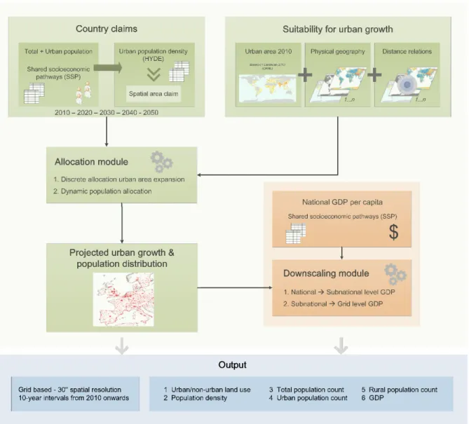
Projections of global population distribution and urbanization become increasingly important in scenario-based assessments of future climate related exposure and vulnerability. According to the UN World Population Prospects, the global population becomes increasingly urban, which triggers the worldwide expansion of urban areas. In recent years, global datasets of gridded population distribution have been developed. These are often characterised by having a relatively coarse spatial resolution of 5-10 km. The methods used simply scaled or extrapolated existing spatial patterns and population densities. The 2UP model is developed to simulate future urban growth and population distribution on a global scale. It includes specific allocation procedures to explicitly account for urban population density change and urban expansion. Besides the simulation of future change in population and urban area, the model is also used to disaggregate national level GDP scenarios. Both the population and GDP scenarios are provided by the Shared Socioeconomic Pathways. Figure 1 shows the conceptual model of 2UP. The basics of the model are similar to other spatial models like the Land Use Scanner (Loonen and Koomen, 2009).

The resulting spatially explicit projections of population growth and urban expansion have a relatively high resolution of 1 kilometre near the equator. To the best of our knowledge, it provides the most detailed global urban growth scenarios that are currently available. The maps illustrate the spectrum of possible (urban) population growth scenarios up to 2050. Overall, they can be applied for the assessment of global flood risks, and they are potentially useful to facilitate ongoing research on global change. As part of the project Vulnerability of

global cities the outcomes will be applied in the Aqueduct Global Flood Analyzer

(http://floods.wri.org). The World Resources Institute (WRI), together with Deltares, VU University Amsterdam, Utrecht University, and PBL Netherlands Environmental Assessment Agency, is working on the development of this online instrument that can measure flood risks at a global level. It is designed for the detailed assessment of global flood risk and will allow users to prioritize where in the world attention to flood risk and flood risk adaptation is needed. Also, it provides country estimates of the costs and benefits of disaster risk reduction strategies.

This background report is written with the intention to qualitatively describe the 2UP model, and is aimed at giving insight into the design of the model and how it is implemented. It includes descriptions of input and the interactions between model components in relation to the calculation procedures used in the model. Also, the assumptions and choices that were made during the development of the model are described. By way of illustration, a few examples of the model output are presented in the last chapter.

(5)

(6)

2 Methodology

2.1 Model input and preparation

2.1.1 Projected population, urbanization and GDP

The Shared Socioeconomic Pathways (SSP) have been developed by the research community to facilitate integrated assessments of climate impacts, vulnerabilities, adaptation and mitigation. They provide possible pathways of society and related societal systems for the 21st century. The SSP projections, five in total, are quantified and documented in the SSP database, and include scenarios for population, urbanization and GDP on global and national scales. The national population data are based on the projection of the International Institute for Applied Systems Analysis – Wittgenstein Centre for Demography and Global Human Capital (IIASA-WIC). The projection data on urbanization are developed by the National Center of Atmospheric Research (Jiang and O’Neill, 2017). The complete database is made publicly available by IIASA (IIASA, 2013). Additional information and references to supplementary material can be found at https://tntcat.iiasa.ac.at/SspDb. Countries are considered and denoted by an ISO 3166-1 alpha3 three-letter country code.

The SSP scenarios provide a suitable starting point for the development of spatial distribution projections of population and exposure of assets to natural hazards. The database contains data for 194 countries from 2010 to 2100. For this project specifically, the population projections were used to extract total and urban population for the period 202050 in 10-year intervals. Also, GDP per capita was extracted for the GDP projections. For this study, only SSP1, 2 and 3 were considered relevant. SSP2 represents a ‘business as usual’ development path. SSP1 and 3 were chosen because their narratives tell an opposing development path relative to SSP2 regarding population growth, urbanization and economic development. Detailed descriptions of the SSP scenarios can be found in e.g. Jiang and O’Neill (2017) and O’Neill et al. (2017).

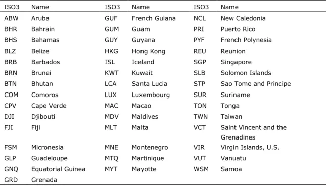
For 43 countries (see table 1) in the SSP database, the population and GDP projections are available but not the urbanization projections. In order to still be able to simulate urban growth for these countries, additional data is used to fill this gap. For these countries the proportion of the total population that is considered urban in 2010, the urban share, is derived from the GRUMP urban extent grid (Balk et al. 2006; CIESIN et al. 2011) in combination with LandScan gridded population count (Bright et al. 2013). The urban share is determined by superimposing the urban extent on the gridded population map and extract the proportion urban population in each country. For the future time steps (2020-2050) the urban share is kept constant for these cases and assumed to be equal to the base year.

2.1.2 Spatial base grid

A spatial base grid with the desired spatial projection and resolution is essential for developing distributed population and land use maps. Consistent with the available flood hazard layers in the Aqueduct Flood Risk Analyzer, the base grid is set up with a spatial resolution of 30 arc seconds (approximately 1 km near the earth’s equator) and spatially referenced to WGS84. Its geographical extent ranges from -180˚E to 180˚W and -90˚S and 90˚N.

(7)

Table 1: Countries (ISO3) with constant urban share

In 2UP the based grid is linked to a country grid, primarily derived from the Global Administrative Areas dataset (GADM, 2012) which includes the common country identification to the ISO 3166-1 standard. This ensures that each country can be identified with means of a country ID. A few country boundaries were manually modified in ArcMap to match the UN country definitions as used by IIASA in the SSP database; GIS-technically Kosovo is included under Serbia; South and North Sudan are joined into one country. For 57 countries, often small countries, subparts of a country or islands, there is no data available in the SSP database and their values are set to NODATA in the modelling process (see table 2).

The spatial base grid originally includes only the cells that consist of 100% land or mainly land when gridded from vector. However, at 30’’ resolution many coastal cells only partly contain land and are thus not included in the original base grid. This grid is therefore extended with those cells that include both part land (however small it is) and water. An additional data layer with land percentage per grid cell is used for this purpose (provided by Deltares: https://aqua-monitor.appspot.com/). The resulting grid includes all cells that are located completely inside or at the boundary of the original country grid. 100% water cells that represent oceans, seas and lakes are left out of the base grid.

For calculating densities (e.g. population density), the model transforms the spatial base grid in an area grid. The area (km2_{) is corrected for latitude, as the actual area of the gridcells}

decreases with increasing latitude north and south of the equator. The area is also corrected for the available land in a grid cell, based on the land percentage per grid cell. Consequently, area represents the area land per grid cell. The model takes this area unit into account in the allocation process of urban area and population. This step prevents the population counts from becoming too high and unrealistic in grid cells where the land percentage is smaller than 100 percent.

ISO3 Name ISO3 Name ISO3 Name

ABW Aruba GUF French Guiana NCL New Caledonia

BHR Bahrain GUM Guam PRI Puerto Rico

BHS Bahamas GUY Guyana PYF French Polynesia

BLZ Belize HKG Hong Kong REU Reunion

BRB Barbados ISL Iceland SGP Singapore

BRN Brunei KWT Kuwait SLB Solomon Islands

BTN Bhutan LCA Santa Lucia STP Sao Tome and Principe

COM Comoros LUX Luxembourg SUR Suriname

CPV Cape Verde MAC Macao TON Tonga

DJI Djibouti MDV Maldives TWN Taiwan

FJI Fiji MLT Malta VCT Saint Vincent and the

Grenadines

FSM Micronesia MNE Montenegro VIR Virgin Islands, U.S.

GLP Guadeloupe MTQ Martinique VUT Vanuatu

GNQ Equatorial Guinea MYT Mayotte WSM Samoa

(8)

Table 2: Countries (ISO3) not modelled within 2UP

2.1.3 Baseline gridded population and urban area

To start the simulation of future urban development from 2010 onwards, first an initial set of global baseline maps of population distribution and urban land use is required. Over the years such datasets have increasingly become available. However, at the time of development none of them appeared to be suitable for this projects’ purpose. Existing maps of global population distribution either lacked the spatial specification for the urban and rural division, or did not meet the requirement that the population input data used needs to be consistent with the reported numbers in the SSP database. Therefore, several freely available data sources are combined to model the baseline population distribution and the urban extent.

During the process of model development and usage, three different methods to create the baseline maps evolved with progressive insight. All three methods are implemented and can be applied when using the model. The methods are briefly described below. Method 2 and 3 make use of an additional data layer containing global urban contours. For the purpose of understanding, its development and use are described first.

Development of urban contours

The urban population shares in the SSP database are adopted from statistics reported by each country individually. Thereby, there is no consistent international definition of “urban” as each country has its own classification to identify urban population based on criteria that include a combination of population size and density, economic activity and physical characteristics. For example, Belgium defines urban as “All the communes which are not part of the list of rural

ISO3 Name ISO3 Name ISO3 Name

ALA Åland FLK Falkland Islands PCN Pitcairn Islands

ASM American Samoa FRO Faroe Islands SHN Saint Helena

AND Andorra ATF French Southern

Territories

KNA Saint Kitts and Nevis

AIA Anguilla GIB Gibraltar SPM Saint Pierre and Miquelon

ATA Antarctica GRL Greenland BLM Saint-Barthélemy

ATG Antigua and Barbuda GGY Guernsey MAF Saint-Martin

BMU Bermuda HMD Heard Island and

McDonald Islands

SMR San Marino BES Bonaire, Saint

Eustatius and Saba

IMN Isle of Man SYC Seychelles

BVT Bouvet Island JEY Jersey SMX Sint Maarten

IOT British Indian Ocean Territory

KIR Kiribati SGS South Georgia and the South Sandwich Islands

VGB British Virgin Islands LIE Liechtenstein SP- Spratly islands

CA- Caspian Sea MHL Marshall Islands SJM Svalbard and Jan Mayen

CYM Cayman Islands MCO Monaco TKL Tokelau

CXR Christmas Island MSR Montserrat TCA Turks and Caicos Islands

CL- Clipperton Island NRU Nauru TUV Tuvalu

CCK Cocos Islands NIU Niue UMI United States Minor Outlying

Islands COK Cook Islands NFK Norfolk Island VAT Vatican City

CUW Curaçao MNP Northern Mariana

Islands

WLF Wallis and Futuna

(9)

communes are considered as urban communes. There are 33 communes which are considered rural…”. The result is that Belgium’s urban population share is 91% and a large part of its territory could be classified as urban land use in the baseline map. The consequence of adhering to the SSP urban shares, the inherent variations in definition of urban population and area are reflected in the baseline urban land use map, which in turn impairs the global comparability of the distribution of urban land use. This hinders the aim of the Aqueduct Flood Risk Analyzer to allow evaluation and comparison of flood risk across countries.

To deal with this challenge and to be able to model urbanization in a consistent manner and provide an operational definition of “urban”, an additional data source is included in the development of the baseline maps. In October 2016 the Global Human Settlement layer (GHSL), developed by the Joint Research Centre (JRC) became available (http://ghsl.jrc.ec.europa.eu/). The GHSL data collection provides accurate spatially detailed and consistent urban land use and population maps and proofed to be particularly useful in modelling the urban extent for the baseline maps from which the future projections can be simulated.

The GHSL is a world-complete data collection that was developed using open satellite data records. In this framework, historical records of Landsat Imagery are organized in four collections (1975, 1990, 2000, and 2014) at 15m, 30m, and 60m spatial resolution, and processed with various sensor characteristics. The satellite imagery is modelled into built up areas (Pesaresi et al. 2015). This layer represents the proportion of built up area within the total size of the grid cell (continues value), and is freely available at 38m, 250m and 1km spatial resolution.

The GHS BUILT-UP map at 38m spatial resolution is used for further processing, with the aim to develop a globally consistent urban land use map. For this, the original built-up presence map is transformed into a discrete urban/non-urban land use map. This reclassification step was done by applying a cap at 50% built-up presence. In words, the grid cells containing 50% or more built-up area are classified as urban land use. This break value is based on visual comparison and correspondence with other high resolution satellite imagery of built up area. Next, the map (Spherical Mercator) is resampled to 30 arcseconds (WGS84) to match with the spatial resolution of the other input maps within the GeoDMS-framework-software.

By including the global urban land use map, an independent and more accurate allocation of urban and rural land use is made possible. By using satellite imagery the result is consistent across countries, and independent of the prescribed definition of urban by countries, allowing for global comparison.

Method 1 (M1)

The 2010 urban population map is created by distributing the country-specific urban share of the SSP total population 2010 proportionally to the ORNL LandScan 2010 population count map (Bright et al. 2011), starting at the highest population count, until the urban total is reached. The resulting extent of urban population is classified as urban land use and the outcome represents the baseline urban land use map. These steps are repeated for the remaining population, representing rural population, and for the surrounding rural (non-urban) land use. Both maps sum up to the total population count.

Method 2 (M2)

The country-specific urban share of the SSP total population 2010 is distributed within the contours of the urban land use map, proportionally to the LandScan 2010 population map. This results in a baseline urban population map. These steps are repeated for the remaining population, representing rural population, and for the surrounding rural (non-urban) land use. Both maps sum up to the total population count.

(10)

Method 3 (M3)

This method makes use of the urban land use map to determine the urban/rural population split. Only the SSP total population is conserved. First, the total population count map is created by distributing the country-specific SSP total population 2010 proportionally to the LandScan 2010 map. The country totals are consistent with the SSP data.

To create the baseline urban population map, the urban land use map is superimposed on the total population count map to make the division between urban area/population and rural area/population. Consequently, the urban population numbers in the SSP database are not used directly. Instead, the relative growth derived from the urban shares in the SSP database is used to simulate future development of the urban population. This means only the SSP country totals are conserved in the baseline, but not the imposed urban/rural population division. Aggregated urban population in the future gridded projections could therefore deviate from the absolute reported numbers in the SSP database.

The advantage of Method 1 and 2 is that by adhering to the urban and rural population division reported by the SSP database, both for the baseline and future projections, aggregated totals by country remain comparable to other studies that make use of the same population projections. Method 3, on the other hand, has the advantage that the global consistency of urban land use allows the comparison between countries. For this reason, the Aqueduct Flood Risk Analyzer has implemented the model outcomes based on method 3.

2.1.4 Projected urban density change

In order to simulate future urban expansion in a spatially explicit manner, the model requires data on the projected spatial growth of urban areas. The SSP database does not contain data on future urban growth or a similar indicator like urban density. Therefore, an additional database was found to fill this gap. The History Database of the Global Environment (HYDE 3.2) contains estimates of mean urban population density per country from 10000 BC to 2100 AD (Klein Goldewijk et al. 2010, 2017; Klein Goldewijk, 2017). It includes data for all SSP scenarios. The urban population density estimates can be used to derive scenario specific national claims for urban area for the period 2010-2100.

The country-specific urban population densities are not used directly in the model, because the numbers do not exactly match with the baseline urban population map. For this reason, the densities are transformed and used as an index so that the course of urban population density over time follows the original data in HYDE. To develop the indices for each SSP scenario and country, the time series with absolute numbers of mean urban population density are converted into an index series with base 2010 == 1. To derive the urban area claim per country in a time step, the corresponding national urban population is divided by the country-specific baseline urban population density of the former time step and corrected by the index. The latter ensures that when the urban population density in a country is projected to decline, the urban area claim increases, provided that there is a projected population increase. In this way, urban sprawl can be simulated with the model. Similarly, densification of urban areas is modelled in case of increasing population density.

(11)

2.2 Drivers of urban growth and spatial analysis

To spatially simulate urban growth, the model requires spatial data of urban drivers; explanatory variables which relate to the processes involved with urban expansion. The qualification of these drivers underlying the spatial patterns of urban growth, and the quantification of these relations are both studies on their own. Past studies have identified several drivers of urban growth and are typically used in urban growth models (Santé et al. 2010). For this project a spatial dataset is collected representing a number of explanatory variables for which it is widely accepted they have influence on urban growth and population distribution. Their characteristics are described below. In the process of selecting the variables, they needed to be available, or easily calculated, on global level and with sufficient spatial resolution, as the objective of the model is to simulate global urban growth at a high resolution. Even though policy-related factors are considered significant drivers of urban expansion (Barredo and Demicheli, 2003; Braimoh and Onishi, 2007), these data were not readily available on a global scale and they are therefore not included in the 2UP model.

2.2.1 Pre-processing of explanatory variables

Although elevation and slope are both often referred to and used as explanatory variables for spatial patterns of urban growth, with grid cells covering approximately 1 km2_{these variables}

might not be as indicative on this scale. Flat terrain at high elevations could be equally suitable for urban area development as low elevated terrain. Also, the average slope of an area aggregated to 1 km2_{is rather coarse for explaining suitability for urban growth. Terrain}

heterogeneity, which describes a combination of heights and multi-directional slopes within an area could contain more information on the suitability for urban growth. Therefore, the Terrain Roughness Index (TRI), an index that quantifies terrain heterogeneity, is used as covariate in the suitability mapping. TRI is calculated according to the method described by Riley et al. (1999), using a high resolution DEM. For this purpose a composite of SRTM V3 (Jarvis et al., 2006) and GTOPO30 (USGS, 1996) elevation data was used. The SRTM V3 elevation map covers the globe between -60 and 60 degrees latitude, and is available with a spatial resolution of 1 arc second (approximately 30 m). The GTOPO (30 arc second resolution) map was used to complete the elevation map for +/- 60-90 degrees latitude by means of linear interpolation between known points in the grid. The resulting TRI map is processed at 30m resolution, with each grid cell containing a discrete index value for terrain roughness. To implement this map into the model it needed to be aggregated to 30 arcseconds. To avoid loss of detail as much as possible, for each TRI class (1-7) a map is compiled by counting the presence of that index value in the coarser grid cell. The seven maps in total are read into the model.

Travel time to the nearest city centre is also considered an explanatory variable of urban growth and population distribution. A map with travel time (in minutes) to the nearest urban centre was derived from a distance analysis based on road density and settlement data. The Global Roads Inventory Project (GRIP) dataset v1 (PBL, 2009) was used, which contains a global road network. Populated places with more than 50,000 inhabitants were used as settlement map.

Distance to urban area and distance to coast are also included in the 2UP model as covariates of urban growth. Both are based on the presence of surrounding urban land use, the latter also in combination with the proximity of the coastline. Future urban area, as well as these two derived variables are endogenously modelled in 2UP. For the spatial analysis, both distance variables are calculated for the baseline urban land use map (2010).

(12)

2.2.2 Spatial analysis

The spatial allocation of urban land use and population distribution to the grid level is based on local suitability for urban land use and population growth. Suitability here can be considered as a proxy for the attractiveness at a location to attract or repel urban area and/or population, based on a set of physical and socio-economic characteristics. The suitability can be determined by quantifying the relation between the explanatory variables and urban land use. For this project, this is done using an inductive approach; the suitability is determined empirically with the aid of a spatial analysis using historical data of urban land use.

The Atlas of Urban Expansion of the Lincoln Institute of Land Policy provides maps that represent urban land cover change between circa 1990 and circa 2000 for a sample of 120 cities across the globe with more than 100,000 inhabitants and distributed over nine world regions (Angel et al. 2012). The urban land use for each city, with a spatial resolution of 30 meters, was derived from Landsat images for the two time steps (Angel et al. 2005).

For the spatial analysis, the set of explanatory variables are superimposed on the urban land use for each city, and their corresponding values are extracted for each urban grid cell. Urban area for both time steps is taken into consideration, except for the analysis with distance to built-up area. Here, only the urban area that was built between the two time periods is used; urban area around 1990 is used as urban contour to determine the distance between newly built and existing urban area.

In the next step, histograms were plotted for each explanatory variable. In this way the relations between urban area and the covariates can be made visible. They all show an inverse relation, which implies that with higher values of terrain roughness, travel time, distance to urban area and coast, the abundance of (new) urban grid cells decreases. The relations that are found can be translated into probability frequency distributions. Only a few points are actually used from these distributions, as the resolution of 30 arsceconds is much coarser compared to the 30 meter resolution from which the relations were derived. This data is used in the 2UP model to transform the explanatory maps into suitability maps.

Inherently to simulating land use forward in time, there is no other way than to assume constant relations between the geographical covariates and future urban growth. Therefore, the distribution of future urban area and population is, at least, partly based on the relations that were found in the historical spatial analysis.

Although the Lincoln dataset is rather limited in global and temporal coverage, at the time of analysis it was the only source of urban area that included multiple time steps that was readily available. Since the release of the Global Human Settlement Layer, which includes four historical time steps and covers much of the world, the spatial analysis was repeated. The results show similar relations between the explanatory variables and historical urban land use.

(13)

2.2.3 Model calibration

To ensure a more solid basis for simulating urban growth an additional, an advanced calibration procedure was carried out by Vrije Universiteit Amsterdam. They applied a statistics-based calibration procedure that links the historical urban land use patterns to the spatially explicit drivers of urban development, using the same global set of explanatory maps as in the spatial analysis (Andree and Koomen, 2017). The statistical analysis estimates the importance of this set of drivers for explaining historical urban land use. This assessment can be used to create the suitability maps that are needed in the model to simulate urban growth.

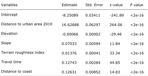
In general, the results show that all explanatory variables significantly contribute to the prediction of urban area at a certain location, the most important driver being distance to urban area. The output of the regression analysis is used in the 2UP model to define the suitability maps and calibrate the urban growth simulation. This is helpful in generating plausible simulation results with the model. Further details of the applied method and discussion of the results can be found in the report by Andree and Koomen (2017).

2.2.4 Model validation

Data from the Global Human Settlement Layer (http://ghsl.jrc.ec.europa.eu/) from the JRC was used for validation of the model representing the past urban area and population. For urban area GHS Built-up grids were taken at the 38 meter resolution level for 1990, 2000 and 2014 and resampled to 30 arcseconds. A limit of 50 percent was taken to be considered as urban area. Population was derived from the GHS population grids at 1km resolution for 1990, 2000 and 2015. Claims for population per country were determined by summing the population in urban areas and released in the model.

The same set of driving forces and relations have been used in the validation as in the model for calculations for the future. The distance to built-up area is considered endogenous, all other factors (Protected areas, Travel Time, TRI) were considered to be static. The index of HYDE-curves was also used as the SSP-scenarios are also differentiating in the past with regard to mean population density.

The model was runned for 25 years from 1990 to 2015 and the allocated urban area was compared with the 2014 urban area map. Visual comparison showed that the modelled urban areas were less patchy compared to the 2014 urban area map. A more quantitative approach was done by raster overlaying (sometimes called combining) of the 1990, 2014 and modelled 2015 map. It showed at a worldwide scale a quite low percentage (depending on the scenario) of changed cells were modelled correctly related to the location. Despite these low percentages the general location of the urban cells were predicted quite well. For population comparison, the widely accepted ANOVA-method was used.

(14)

2.3 Future distribution of urban area and population

The core of the 2UP model and its primary objective is to disaggregate the scenario-based projected national-level urban population to 30 arcseconds and simulate urban expansion for 194 countries and territories. Starting with the urban population baseline map, the modelling process consist of 3 main steps: (1) calculate the suitability representing the relative attractiveness for urban growth of each grid cell, (2) allocate projected urban area to grid cells in a country, and (3) disaggregate projected urban population change to urban grid cells. The modelling steps are repeated for each 10 year time interval and SSP. The model procedures are explained in more detail below.

2UP is based on the Geo Data and Model Server (GeoDMS) modelling framework. This is an open source and flexible calculating engine that allows the handling, calculation and visualization of geographical data varying in resolution and extent. GeoDMS is particularly useful for global-scale modelling as it can handle large spatial grid-datasets and calculates relatively fast. It has the advantage that functionalities specifically for land use change modelling and allocation procedures are already built-in. Furthermore, its use has been proven in several land use modelling projects for the Netherlands and Europe, Land Use Scanner and EU CLUE Scanner respectively (e.g. Hilferink and Rietveld, 1999; Koomen and Borsboom-van Beurden, 2011; Lavalle et al. 2011). The framework is developed and made freely available by Object Vison (http://www.objectvision.nl/).

In general, the land surface on earth is not considered completely habitable for population settlement. For this reason, a land mask is constructed from multiple spatial data layers to exclude unsuitable grid cells for habitation. This mask is processed by overlaying the following data layers: surface water and permanent snow and ice cover. The Water Bodies Map dataset from the ESA Land Cover Climate Change Initiative (Defourny, 2016) is used to mask global surface water. Permanent snow and ice cover is extracted from the MODIS Collection 4 global land cover dataset (Friedl et al. 2002) and these areas are excluded from the allocable land as well. The so-called ‘FreeLand’ is left over in the model as allocable. The processing of the baseline data (section 2.1.3) did not account for the excluded land described above. As a consequence, some slight overlap existed between the baseline urban land use and population maps, and the excluded grid cells. For modelling purposes, the baseline maps were kept as is. However, in the modelling process the excluded grid cells are omitted from receiving projected urban area and population growth.

2.3.1 Suitability mapping

Suitability represents the relative attractiveness for urban land use and population, and is used in the model to simulate urban growth. The global set of explanatory variables (section 2.2), provides the basis for creating the suitability maps, and is loaded into the model. With use of the probability frequency distributions that are derived from this spatial analysis based on historical urban land use (section 2.2.2), the variables are transformed into suitability maps. First, the probability distributions are read into the model as table. Then the explanatory variable maps are re-classified using the corresponding probability values.

The seven maps with TRI, one for each TRI class, containing the frequency of the index values per 30’’ grid cell, are combined into one suitability map. This is done by multiplying the probability and the frequency values for each TRI class, and add them together in one map. The variables distance to urban area and coast are endogenously calculated within the model. Distance to urban area is an indicator based on the presence of urban land use at a location and its surroundings. It is calculated by taking the sum of the total amount of urban area in the neighbouring grid cells after applying a relative weight based on their distance to the central grid cell. The weight quickly decreases with increasing distance. The number of neighbouring cells that can contribute to this potential of each cell is restrained by applying a

(15)

buffer of ±10 kilometres. Distance to coast is calculated similarly as distance to urban area, and used as an indicator of urban suitability. It is based on a combination of urban area and its distance to the coastline. The potential for urban area within a distance of 20 kilometres of the coast is considered higher than urban areas outsides this range. So, the weight of potential for urban area decreases with distance to the coast.

The relative contribution of the individual suitability maps determines the total suitability at a location, which is eventually used in the allocation process. There are several approaches to weigh the suitability maps. One is to use expert judgement in combination with testing model behaviour. The second method is more robust and makes use of the calibrated regression coefficients from the calibration output (section 2.2.3). Both approaches are implemented in the model and can be applied when using the model.

In case of the first approach, the weights that are given to the suitability maps are based on judgements expressed by experts in the field of land use change modelling and by testing the model behaviour. Distance to urban area was giving the most weight relative to the total suitability. Distance to coast was also given more weight relative to TRI and travel time. The latter two were weighted equally.

The second method creates the final suitability map by adding up the values for the intercept and the local values of the explanatory variables multiplied by their estimated coefficients. The regression coefficients used are presented in Table 3.

Table 3: Regression coefficients (Andree and Koomen, 2017)

2.3.2 Scenario-specific suitability

The spatial distribution of urban expansion and population growth that is simulated by the model, is mainly driven by (1) national level population, (2) national level urbanization, (3) national level urban density change, and (4) suitability mapping. The first three factors are SSP specific and their differences are expressed in the model outcomes. The fourth factor, suitability mapping, is grid-level specific and primarily impacts the within country spatial patterns. However, it is static across the SSP scenarios.

To implement variation between the SSP’s, regarding suitability, two additional geospatial data layers are added to the suitability mapping: Protected land and flood-prone area. For the protected land map the World Database on Protected Areas (WDPA) dataset is used (IUCN, 2009). The flood-prone area map represents river flood extent (100 year return period) and was collected from the GLOFRIS framework (Ward et al. 2013; Winsemius et al. 2013). The

Variables Estimate Std. Error z-value P value

Intercept -8.25089 0.03411 -241.89 <2e-16

Distance to urban area 2010 16.62688 0.06297 264.06 <2e-16

Elevation -0.00066 0.00002 -29.48 <2e-16

Slope 0.07033 0.00594 11.84 <2e-16

Terrain roughness index 0.01376 0.00041 33.34 <2e-16

Travel time 0.12743 0.00284 44.85 <2e-16

Distance to coast 0.12631 0.00852 14.83 <2e-16

(16)

on local suitability for urban growth can be linked to the SSP narratives. SSP1 Sustainability describes a world in which significance is given to environmental protection, innovation and urbanization is well managed. SSP3 Regional Rivalry, on the other hand, pictures a world where low economic growth and innovation leads to little environmental protection and failing spatial planning. In the Middle of the Road (SSP2) scenario, the spatial pattern of development is consistent with historical patterns.

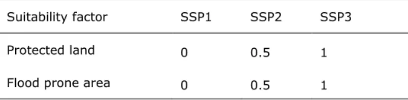
From these narratives, a SSP specific parameter value is deduced to modify local suitability and to account for local differentiation between scenarios. The final suitability is determined by multiplying the parameter value with the local suitability value in case of protected land, flood prone area, or both. Thus, for example, when a grid cell is located within protected land the suitability is set to zero for SSP1 and urban growth is excluded from this area. In table 4 SSP specific parameter values for suitability are presented for each combination of SSP and suitability factor.

Table 4: SSP specific parameter values for suitability

2.3.3 Allocation of urban area

The allocation of urban area within a country is based on the projected urban area claim; derived from the HYDE database (section 2.1.4) and the suitability (by means of mean population density in urban area). For each time step, the projected amount of urban area (claim) is determined and the final suitability map is calculated. Thereafter, the urban area is allocated proportionally to the suitability map. This allocation procedure includes two steps: (1) the suitability within a country is sorted in a descending order, and (2) the urban area is allocated to the grid cells containing the highest suitability until the total claim is met. Both suitability and urban area are discrete across all cells, and as such each cell is either defined as urban or rural. For time step n + 1 the corresponding urban area claim is again entirely allocated.

The allocation accounts for the area of grid cell and the area of available land within a grid cell (section 2.1.2). The base grid also includes grid cells with a percentage of land smaller than 100. Therefore, the area of available land in a grid cell is used as weight in the allocation process. Consequently, the amount of urban area (km2_{) that is allocated to a grid cell depends}

on the actual area of land in a grid cell.

2.3.4 Distribution of population change

The allocation of population is based on the projected population change and suitability. The latter is assumed equal for both the allocation of urban area and population. The model is directed at downscaling urban population and it builds on the simulated urban land use map from the previous step. The distribution is done recursively, which means the urban population allocation in time step n is used in the simulation for time step n+1. Thereby, for each time step the projected change in urban population is allocated within the urban area, and proportionally to the relative distribution of suitability in the urban area. The grid cells with the highest suitability receive a proportionally larger share of the urban population change. Here also the allocation is weighted to the area of available land in a grid cell.

Suitability factor SSP1 SSP2 SSP3

Protected land 0 0.5 1

(17)

In more detail, the allocation procedure of urban population for each time step includes the following steps:

1. The projected change in urban population in a country is calculated, which determines if there is a growth or decline of population.

2. The suitability within the allocated urban area is calculated.

3. A maximum urban population density is set for each grid cell. This maximum is based on the urban population in that grid cell and its surroundings. It is calculated by taking the total sum of urban population and its neighbouring cells in a perimeter of ±10 kilometres after applying a relative weight based on their distance to the central grid cell.

4. To prevent that either very low or very high maximum densities are calculated, respectively the minimum and maximum density are constrained. To ensure urban population is able to grow in low density urban areas, the bottom limit is set by taking the mean urban population density in a country. On the other hand, exceptional growth in highly populated urban areas will be restricted by the maximum urban population density calculated at step 3. The mean urban density is calculated by multiplying the urban population density of a country with the corresponding HYDE index (see section 2.1.4).

5. The urban population change, calculated in step 1, is allocated to the urban area and proportionally to the suitability within the urban area. This is an iterative process; population is allocated to grid cells with the highest suitability for which the maximum density is not yet reached and continues until the national-level urban population claim is met.

6. In case there is projected population decline in a country, the suitability within the urban area is inverted. This makes sure the depopulation will occur at the fringes of the urban areas first before the city centres.

The remaining rural population is also disaggregated to the grid level. Because the model is not aimed at the simulation of developments in rural area and population, this is done in a straightforward way. The projected national-level rural population is distributed proportionally to the population distribution of LandScan 2010 (Bright et al. 2010). Rural population is only allocated to none-urban areas.

2.3.5 Disaggregation of GDP projections

When presented on global scale, most datasets on economic development are still available mainly at national level. For spatial analysis, the national figures are often disaggregated to the grid-level according to population density across a country. Only recently such data can also be found on sub-national scale, which makes it possible to achieve higher precision than country scale. Gennaioli et al. (2012) developed a sub-national dataset (tabulated) which includes Gross Domestic Product (GDP) per capita in constant 2005 international USD. The database consist of 1569 sub-national regions (i.e. province, state etc. depending on country in question) across 110 countries. Although sub-national GDP data is missing for most of the African continent, the data covers 74% of the world’s land surface and 96% of its GDP. The temporal coverage is also country specific and ranges from 1960-2010.

Disaggregation of the national GDP projections to the grid-level is based on the sub-national data from this dataset whenever possible, in combination with national data from the SSP database. In this way the spatial variation in economic development within countries is taken

(18)

The table with GDP per capita data was spatially joined with the country base grid, based on GADM country boundaries. Because the latter also includes first level administrative sub-national boundaries, the regional GDP data could therefore be linked to the base grid. The division of sub-national regions in the original database did not perfectly match the regional division in the GADM base grid. Therefore, several manual adjustments were necessary to correct for these deviations. In this process, lower level subdivision of regions in the original data needed to be aggregated to one region in the base grid in some cases. Consequently, the number of sub-national regions in the end result is lower, but the coverage remained the same. When available, the reported regional value for GDP per capita for 2010 is used, followed by the most recent year in the sub-national database. In case of a missing value, national GDP per capita (SSP database) is used to fill the gaps.

The following calculation steps are included in the disaggregation process:

1. For the development of the baseline grid for 2010, the first step is to assign sub-national GDP per capita to the corresponding regions of the base grid. If there is no data for a region, the national GDP per capita is assigned to that region. If no regional data is available at all, then national GDP per capita is assigned to every region in that country. 2. The sub-national GDP per capita is not used directly but as an index to scale the national

GDP per capita within a country. This ensures that the national GDP figures as reported by the SSP database are conserved. To derive the index values for each region, the ratio between the sub-national GDP per capita and the national GDP per capita is calculated. 3. The sub-national GDP is then calculated by multiplying the national GDP per capita

reported by the SSP database with gridded population count (section 2.3.4), and by the calculated index value (step 2) to correct for the regional differences within a country. 4. To ensure consistency between the national and sub-national data, the sub-national GDP

needs to be corrected by the ratio between national GDP and the sum of the sub-national GDP in a country. In this way the sum of sub-national GDP equals the total GDP of a country as reported by the SSP database.

5. Steps 2 to 4 are repeated for each successive time step, and for each SSP. The future development of sub-national GDP is based on the growth factor of national GDP per capita between two successive years in the SSP database. For time step n + 1, sub-national GDP per capita is calculated by multiplying the growth factor with sub-national GDP per capita at time step n.

The final global grids represent GDP per grid cell. They include a combination of sub-national data whenever possible, and national GDP figures in case of missing data.

(19)

3 Results

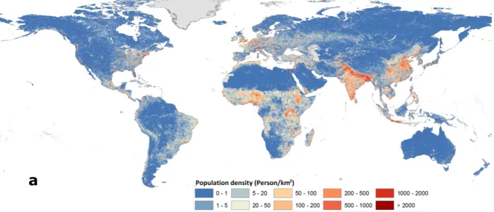
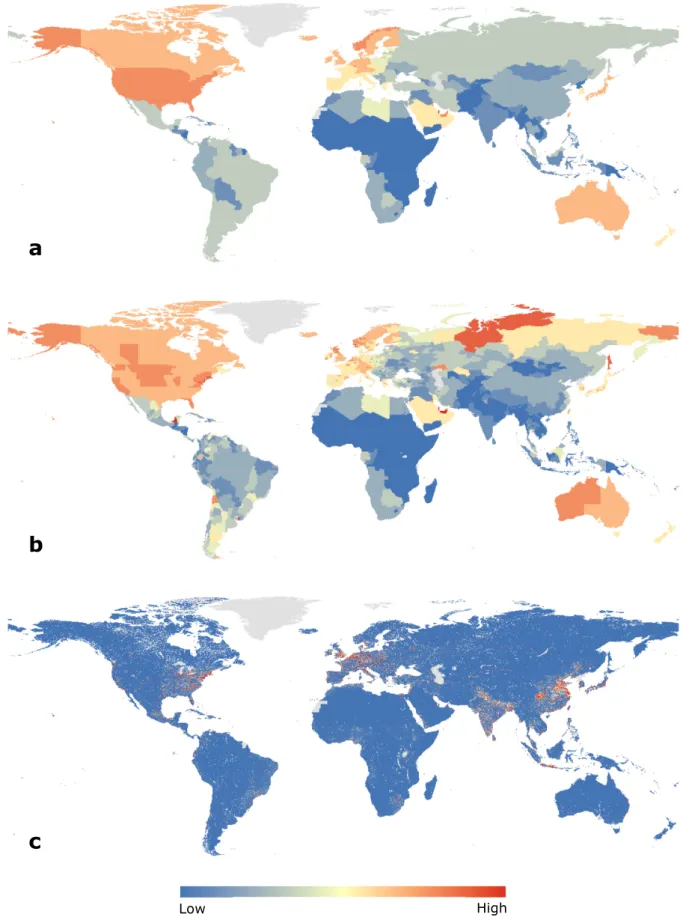
In this chapter, a few examples are presented which illustrate the outcomes of the 2UP model. The spatially explicit global projections of population growth (Figure 2) and Gross Domestic Product (Figure 3) are a necessary component in the assessment of exposure and vulnerability to hazards. The outcomes of 2UP are a step forward in global scale spatially explicit population and GDP scenarios, and they are potentially very useful to facilitate ongoing global change research.

3.1 Global projections of population growth

Figure 2. (a) Projected population density for SSP2 (2050), and (b) corresponding

a

b

Decline Growth Population

(20)

3.2 Global projections of Gross Domestic Product

Figure 3. Downscaling projected GDP from (a) national to (b) subnational, and (c) grid level

a

b

c

(21)

4 References

Andree, B.P.J. and Koomen, E., 2017. Calibration of the 2UP model: Spinlab Research Memorandum SL-13. Vrije Universiteit Amsterdam.

Angel, S., Sheppard, SC., Civco, DL., Buckley, R., Chabaeva, A., Gitlin, L., Kraley, A., Parent, J., Perlin, M., 2005. The dynamics of global urban expansion. Transport and Urban

Development Department, The World Bank.

[dataset ] Angel, S., Parent, J., Civco, D.L., and Blei, A.M., 2012. Atlas of urban expansion. Cambridge, MA: Lincoln Institute of Land Policy. Available at

http://datatoolkits.lincolninst.edu/subcenters/atlas-urban-expansion/

Balk, D.L., Deichmann, U., Yetman, G., Pozzi, F., Hay, S.I., and Nelson, A., 2006.

Determining Global Population Distribution: Methods, Applications and Data. Advances in Parasitology, 62, 119-156, doi:10.1016/S0065-308X(05)62004-0.

Barredo, J.I. and Demicheli, L., 2003. Urban sustainability in developing countries’ megacities: modelling and predicting future urban growth in Lagos. Cities, 20(5), 297– 310, doi: 10.1016/s0264-2751(03)00047-7.

Braimoh, A.K. and Onishi, T., 2007. Spatial determinants of urban land use change in Lagos, Nigeria. Land Use Policy, 24(2), 502–515, doi: 10.1016/j.landusepol.2006.09.001. [dataset] Bright, E.A., Coleman, P.R., Rose, A.N., Urban, M.L., 2011. LandScan 2010 High

Resolution Global Population Data Set. Oak Ridge National Laboratory, TN, US. http://web.ornl.gov/sci/landscan/.

[dataset] Bright, E.A., Coleman, P.R., Rose, A.N., and Oak Ridge National Laboratory, 2013. LandScan Global Population Database 2013. Oak Ridge National Laboratory, UT-Battelle, LLC.

[dataset] Center for International Earth Science Information Network - CIESIN - Columbia University, International Food Policy Research Institute - IFPRI, The World Bank, and Centro Internacional de Agricultura Tropical – CIAT, 2011. Global Rural-Urban Mapping Project, Version 1 (GRUMPv1): Urban Extents Grid. Palisades, NY: NASA Socioeconomic Data and Applications Center (SEDAC), doi:10.7927/H4GH9FVG.

[dataset] Defourny, P., 2016. ESA Land Cover Climate Change Initiative (Land_Cover_cci): Water Bodies Map, v4.0. Centre for Environmental Data Analysis. Available at

http://catalogue.ceda.ac.uk/uuid/7e139108035142a9a1ddd96abcdfff36

[dataset] Friedl, M., McIver, D., Hodges, J. C., Zhang, X., Muchoney, D., Strahler, A., Woodcock, C., Gopal, S., Schneider, A., Cooper, A., Baccini, A., Gao, F. and Schaaf, C., 2002. Global land cover mapping from MODIS: algorithms and early results. Remote Sensing of Environment, 83(1), 287–302, doi: 10.1016/S0034-4257(02)00078-0. [dataset] Global Administrative Areas ( 2012). GADM database of Global Administrative

(22)

Gennaioli, N., La Porta, R., Lopez-de-Silanes, F., and Shleifer, A. 2012. Human capital and regional development. The Quarterly journal of economics, 128(1), 105-164,

doi:10.1093/qje/qjs050.

Hilferink, M. and Rietveld, P., 1999. LAND USE SCANNER: An integrated GIS based model for long term projections of land use in urban and rural areas. Journal of Geographical

Systems, 1(2), 155–177, doi:10.1007/s101090050010.

[dataset] International Institute for Applied Systems Analysis (IIASA), 2013. SSP database. Available at https://tntcat.iiasa.ac.at/SspDb.

[dataset] IUCN, UNEP-WCMC, 2009. The World Database on Protected Areas (WDPA). Cambridge (UK): UNEP World Conservation Monitoring Centre. Available at

www.protectedplanet.net.

[dataset] Jarvis A., Reuter, H.I., Nelson, A., Guevara, E., 2006. Hole-filled SRTM for the globe version 3, from the CGIAR-CSI SRTM 90m database. Available from

http://srtm.csi.cgiar.org.

Jiang, L. and O’Neill, B. C., 2017. Global urbanization projections for the Shared Socioeconomic Pathways. Global Environmental Change, 42, 193-199, doi: 10.1016/J.GLOENVCHA.2015.03.008.

Klein Goldewijk, K., Beusen, A. & Janssen, P., 2010. Long-term dynamic modeling of global population and built-up area in a spatially explicit way: HYDE 3.1. The Holocene, 20(4), 565-573, doi:10.1177/0959683609356587.

[dataset] Klein Goldewijk, Dr. ir. C.G.M. (Utrecht University) 2017: Anthropogenic land-use estimates for the Holocene; HYDE 3.2. DANS. doi:10.17026/dans-25g-gez3.

Klein Goldewijk, K., Beusen, A., Doelman, J. & Stehfest, E., 2017. Anthropogenic land use estimates for the Holocene – HYDE 3.2. Earth System Science Data, 9(2), 927-953, doi: 10.5194/essd-9-927-2017.

Koomen, E., and Borsboom-van Beurden, J. (Eds.), 2011. Land-Use Modelling in Planning Practice. GeoJournal Library. Springer Netherlands. doi:10.1007/978-94-007-1822-7 Lavalle, C., Baranzelli, C., e Silva, F.B., Mubareka, S., Gomes, C.R., Koomen, E., and

Hilferink, M., 2011. A High Resolution Land Use/Cover Modelling Framework for Europe: Introducing the EU-ClueScanner100 Model, in: Computational Science and Its Applications - ICCSA 2011. Springer Berlin Heidelberg, pp. 60–75, doi:10.1007/978-3-642-21928-3_5.

Loonen, W. and Koomen, E., 2009. Calibrating and validating the Land Use Scanner algorithms. Netherlands Environmental Assessment Agency (PBL), The Hague, The Netherlands.

O’Neill, B.C., Kriegler, E., Ebi, K.L., Kemp-Benedict, E., Riahi, K., Rothman, D.S., … Solecki, W., 2017. The roads ahead: Narratives for shared socioeconomic pathways describing world futures in the 21st century. Global Environmental Change, 42, 169–180, doi: 10.1016/j.gloenvcha.2015.01.004.

(23)

[dataset] Planbureau voor de Leefomgeving (PB), 2009. GRIP Global Roads Inventory Project version 1. Available at:

http://geoservice.pbl.nl/website/flexviewer/index.html?config=cfg/PBL_GRIP.xml&center =445277.96317309,6800125.4543973&scale=5000000

[dataset] Pesaresi, M., Ehrilch, D., Florczyk, A. J., Freire, S., Julea, A., Kemper, T., Soille, P., Syrris, V., 2015. GHS built-up grid, derived from Landsat, multitemporal (1975, 1990, 2000, 2014). European Commission, Joint Research Centre (JRC). PID:

http://data.europa.eu/89h/jrc-ghsl-ghs_built_ldsmt_globe_r2015b

Riley, S.J., DeGloria, S.D., and Elliot, S.D., 1999. A terrain ruggedness index that quantifies topographic heterogeneity. International Journal of Science, 5, 23-27.

Santé, I., García, A.M., Miranda, D., and Crecente, R., 2010. Cellular automata models for the simulation of real-world urban processes: A review and analysis. Landscape and Urban Planning, 96(2), 108–122, doi:10.1016/j.landurbplan.2010.03.001.

[dataset] US Geological Survey, 1996. Global Digital Elevation Model (GTOPO30). EROS Data Center Available at https://lta.cr.usgs.gov/GTOPO30.

Ward, P.J., Jongman, B., Weiland, F.S., Bouwman, A., van Beek, R., Bierkens, M.F., Ligtvoet, W., and Winsemius, H.C., 2013. Assessing flood risk at the global scale: model setup, results, and sensitivity. Environmental research letters, 8(4), 44019, doi: 10.1088/1748-9326/8/4/044019.

Winsemius, H.C., Van Beek, L.P.H., Jongman, B., Ward, P.J., and Bouwman, A., 2013. A framework for global river flood risk assessments. Hydrology and Earth System Sciences, 17(5), 1871–1892, doi: 10.5194/hess-17-1871-2013.

Towards an urban preview: Modelling future urban growth with 2UP